5주차 | 딥러닝(Deep learning)(1)

21 Mar 2024 in KT AIVLE SCHOOL

KT AIVLE SCHOOL 5기 5주차에 진행한 딥러닝(Deep learning) 강의 내용 정리 글입니다.

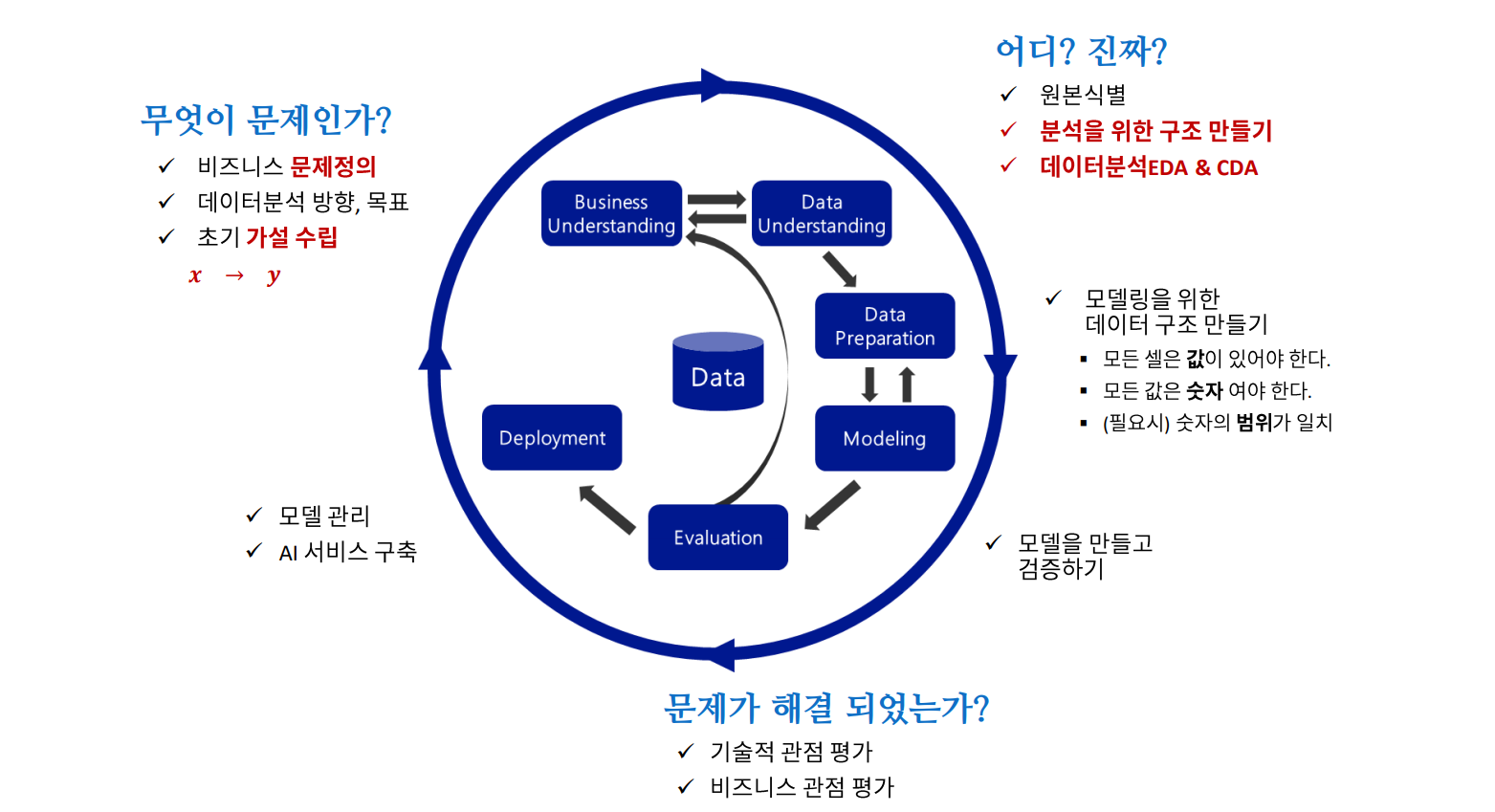
CRISP-DM
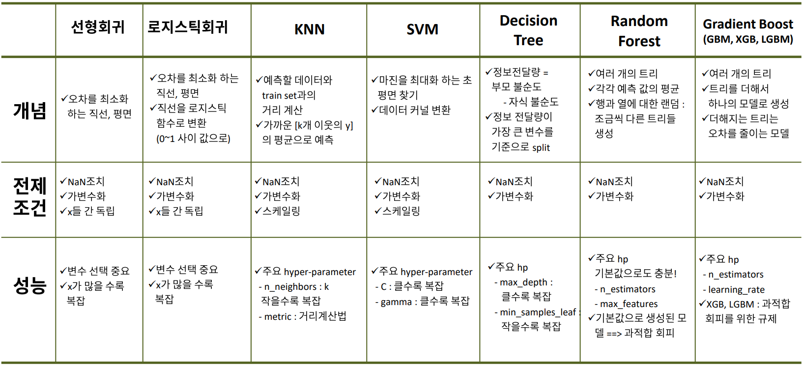
머신러닝 알고리즘 정리
딥러닝 개념 익히기
- 학습 절차
딥러닝 모델링 : 회귀
Feature Representation
- Hidden Layer
딥러닝 모델링: 이진 분류
딥러닝 모델링: 다중 분류
요약
참조

CRISP-DM

Untitled

머신러닝 알고리즘 정리

alt text

딥러닝 개념 익히기

모델링 : 파라미터를 잘 찾는것 → train error를 최소화하는 과정
튜닝 : val error를 최소화하는 과정

학습 절차

어떤 정보 : node 혹은 뉴런(Neuron)
- 어떤 정보에 알맞은 가중치와 절편을 찾아가는 과정
model.fit하는 순간
1. 가중치(파라미터)에 초기값을 할당 (랜덤으로)
2. 예측 결과를 뽑는다
3. 오차를 계산(loss) → forward propagation(순전파)
4. 오차를 줄이는 방향으로 가중치 조정(방향 : optimizer, 얼만큼 : learning rate(중요)) → back propagation(역전파)
5. 다시 1단계로 올라가 반복 (epoch)
하이퍼파라미터 : 머신러닝에서 사람이 개입할 여지
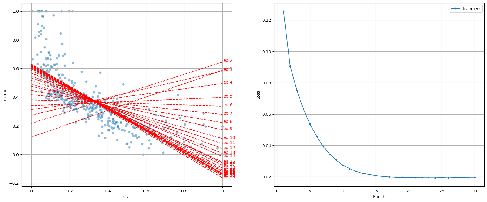
[30번 조정하며 최적의 가중치 찾는 과정]

딥러닝 모델링 : 회귀

딥러닝 과정 및 구조

딥러닝에서 스케일링은 필수
- Normalization(정규화) : 모든 값의 범위를 0 ~ 1로 변환 → 보통 많이 사용
- Standardization(표준화) : 모든 값을 , 평균 = 0, 표준편차 = 1로 변환
Process
- 각 단계(task)는 이전 단계의 output을 input으로 받아 처리한 후 다음 단계로 전달
- 공통의 목표를 달성하기 위해서 동작
- ex) 상품 기획 → 디자인 → 생산 → 물류 입고 → 매장 판매
딥러닝 구조
- Input : 입력되는 x의 분석 단위(Layer 아님)
- Hidden Layer
  - layer 여러개 : 리스트[]로 입력
  - hidden layer
    - input_shape는 첫번째 layer만 필요
    - activation
      - 히든 레이어는 활성함수 필요(보통 ‘relu’ 사용)
  - output layer : 예측 결과가 1개
  - 활성화 함수(Activation Function)
    - 현재 레이어의 결과값을 다음 레이어(연결된 각 노드)로 어떻게 전달할지 결정 변환 해주는 함수
    - 없으면 히든 레이어를 아무리 추가해도 그냥 선형회귀
    - Hidden Layer: 선형함수 → 비선형 (ReLU), Output Layer: 결과값 다른 값으로 변환 (주로 분류 모델에서 필요)
      - Sigmoid, tanh, ReLU(Hidden Layer 국룰)
  - 보통 노드의 수를 점차 줄여간다
- Output Layer
- Output

딥러닝 코드

Dense
- input_shape = ( , ) : 분석 단위에 대한 shape
  - 1차원 : (feature수, ), 2차원 : (rows, cols)
- output : 예측 결과가 1개 변수
Compile
- 선언된 모델에 대해 몇가지 설정을 한 후, 컴퓨터가 이해할 수 있는 형태로 변환하는 작업
- loss function(오차 함수)
  - 오차 계산 무엇으로 할지 결정
  - 회귀는 보통 mse
- optimizer
  - 오차를 최소화 하도록 가중치 조절
  - optimizer = ‘adam’ : learning_rate 기본 값 = 0.001
  - optimizer = Adam(learning_rate = 0.1) : 옵션 값 조정 가능
learning_rate
- 적절하게 조절하는 것이 좋다
학습
- epochs : 반복 횟수 → 전체 데이터를 몇 번 학습
- validation_split = 0.2 → 학습 데이터의 20%를 검증 데이터로 사용
학습 곡선
- .history
  - 학습 수행 과정에 가중치가 업데이트 되면서 그 때 마다의 성능 측정하여 기록
  - 학습 시 계산된 오차 기록(가이드)
- 바람직한 곡선
  - epoch가 증가하면서 loss가 큰 폭으로 축소 후, 점차 loss 감소 폭이 줄어들면서 감소
- 들쑬 날쑥하면서 loss 감소 → learning_rate 줄이기
- val_loss가 줄어들다가 다시 상승(과적합)
  - epoch와 learnig_rate 조절

실습

import pandas as pd
import numpy as np
import matplotlib.pyplot as plt
import seaborn as sns

from sklearn.model_selection import train_test_split
from sklearn.metrics import *
from sklearn.preprocessing import MinMaxScaler

from keras.models import Sequential
from keras.layers import Dense
from keras.backend import clear_session
from tensorflow.keras.optimizers import Adam
#from keras.optimizers import Adam : 버전에 따라 다르다

def dl_history_plot(history):
    plt.figure(figsize=(10,6))
    plt.plot(history['loss'], label='train_err', marker = '.')
    plt.plot(history['val_loss'], label='val_err', marker = '.')

    plt.ylabel('Loss')
    plt.xlabel('Epoch')
    plt.legend()
    plt.grid()
    plt.show()

path = 'https://raw.githubusercontent.com/DA4BAM/dataset/master/boston.csv'
data = pd.read_csv(path)

target = 'medv'
x = data.drop(target, axis = 1)
y = data.loc[:, target]
x_train, x_val, y_train, y_val = train_test_split(x, y, test_size=.2, random_state = 20)

scaler = MinMaxScaler()
x_train = scaler.fit_transform(x_train)
x_val = scaler.transform(x_val)

nfeatures = x_train.shape[1]
model3 = Sequential([  Dense(2, input_shape = (nfeatures,), activation = 'relu'),
                       Dense(1)   ])
model3.summary()
model3.compile( optimizer= Adam(learning_rate=0.08), loss = 'mse')
hist = model3.fit(x_train, y_train, epochs = 50 , validation_split= .2, verbose = 0).history
dl_history_plot(hist)

pred3 = model3.predict(x_val)
print(f'RMSE : {mean_squared_error(y_val, pred3, squared=False)}')
print(f'MAE  : {mean_absolute_error(y_val, pred3)}')
print(f'MAPE : {mean_absolute_percentage_error(y_val, pred3)}')

Feature Representation

Hidden Layer

연결
- 모든 노드 간 연결(Fully Connected)
- 연결 제어(Locally Connected)
학습
- 오차를 계산하고 오차를 줄이기 위해 파라미터(가중치) 업데이트
- 각 노드 별로 값 생성
Hidden Layer 내부에서 발생한 일
- 기존 데이터로 새로운 특징(new feature)를 만듦
- 예측 값과 실제 값 사이의 오차를 최소화 해주는 유익한 특징일 것이다
- 기존 데이터가 새롭게 표현(Representation)되는 Feature Engineering이 진행된 것
Deep Learning → Representation Learning

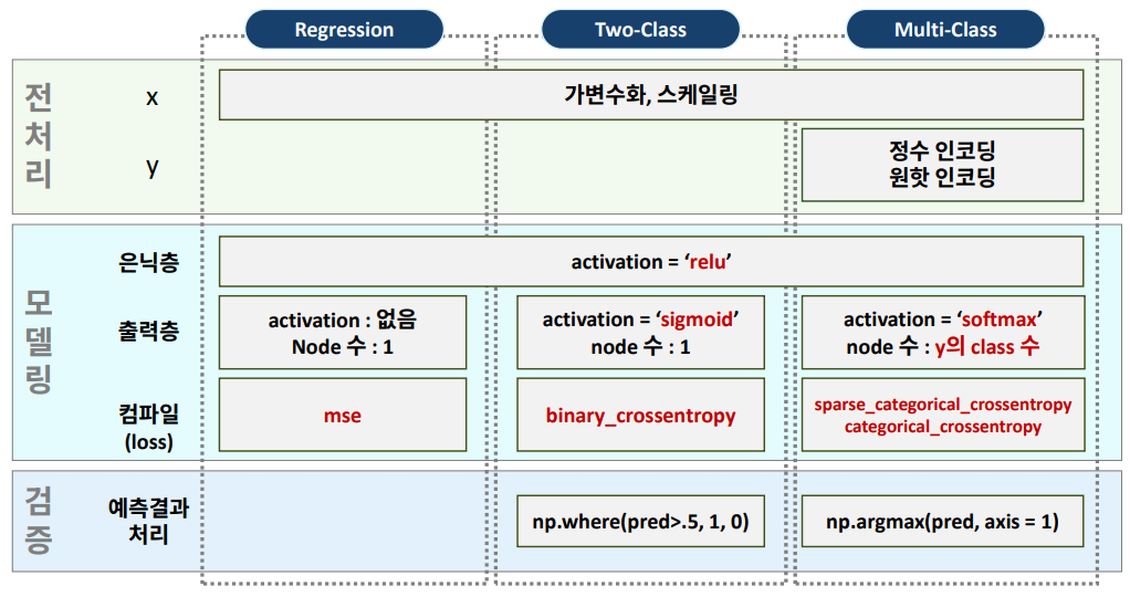
딥러닝 모델링: 이진 분류

결과를 변환시켜줄 활성화 함수가 필요(시그모이드 함수)

활성 함수(Activation Function)

node의 결과를 변환 시켜주는 역할
- Hidden Layer
  - Activation Function : ReLU
  - 기능 : 좀 더 깊이 있는 학습을 시키려고
- Output Layer
  - 회귀 : X
  - 이진 분류
    - Activation Function: sigmoid
    - 기능: 결과를 0, 1로 변환
  - 다중 분류
    - Activation Function: softmax
    - 기능: 각 범주에 대한 결과를 범주별 확률 값으로 변환

Loss Function : binary_crossentropy

이진 분류 모델에서 사용되는 loss function
y=1, y=0 일 때 각각 오차들의 평균

실습

import pandas as pd
import numpy as np
import matplotlib.pyplot as plt
import seaborn as sns

from sklearn.model_selection import train_test_split
from sklearn.metrics import *
from sklearn.preprocessing import MinMaxScaler

from keras.models import Sequential
from keras.layers import Dense
from keras.backend import clear_session
from tensorflow.keras.optimizers import Adam
from imblearn.over_sampling import RandomOverSampler

# 학습곡선 함수
def dl_history_plot(history):
    plt.figure(figsize=(10,6))
    plt.plot(history['loss'], label='train_err', marker = '.')
    plt.plot(history['val_loss'], label='val_err', marker = '.')

    plt.ylabel('Loss')
    plt.xlabel('Epoch')
    plt.legend()
    plt.grid()
    plt.show()
    
path = "https://raw.githubusercontent.com/DA4BAM/dataset/master/Attrition_train_validation.CSV"
data = pd.read_csv(path)
data['Attrition'] = np.where(data['Attrition']=='Yes', 1, 0)

target = 'Attrition'
data.drop('EmployeeNumber', axis = 1, inplace = True)
x = data.drop(target, axis = 1)
y = data.loc[:, target]

dum_cols = ['BusinessTravel','Department','Education','EducationField','EnvironmentSatisfaction','Gender',
            'JobRole', 'JobInvolvement', 'JobSatisfaction', 'MaritalStatus', 'OverTime', 'RelationshipSatisfaction',
            'StockOptionLevel','WorkLifeBalance' ]

x = pd.get_dummies(x, columns = dum_cols ,drop_first = True)

x_train, x_val, y_train, y_val = train_test_split(x, y, test_size = 200, random_state = 2022)

scaler = MinMaxScaler()
x_train = scaler.fit_transform(x_train)
x_val = scaler.transform(x_val)

n = x_train.shape[1]
# 60, 60, 10, 5, 1 
clear_session()
model = Sequential([Dense(60, input_shape = (n, ), activation = 'relu'), 
                           Dense(60, activation = 'relu'), 
                            Dense(10, activation = 'relu'), 
                            Dense(5, activation = 'relu'),
                           Dense(1, activation = 'sigmoid')])
model.summary()

model.compile(optimizer = Adam(learning_rate = 0.001), loss = 'binary_crossentropy')
hist = model.fit(x_train, y_train, epochs = 100, validation_split = 0.2, verbose = 0).history

dl_history_plot(hist)

pred = model.predict(x_val)
pred = np.where(pred >= 0.5, 1, 0)

print(confusion_matrix(y_val, pred))
print(classification_report(y_val, pred))

# resampling
ros = RandomOverSampler()
x_train_ros, y_train_ros = ros.fit_resample(x_train, y_train)
print(y_train_ros.value_counts(normalize = True))
print(y_train_ros.value_counts())

딥러닝 모델링: 다중 분류

Output Layer

Node 수: y의 범주수
Softmax: 각 class 별(Output Node)로 예측한 값을, 하나의 확률 값으로 반환

다중 분류 모델링을 위한 전처리

다중 분류: y가 범주이고, 범주가 3개 이상
방법 1: 정수 인코딩 + sparse_categorical_crossentropy
- y: Integer Encoding → class들을 0부터 시작하여 순차 증가하는 정수로 인코딩
- int_encoder.classes_ → 배열의 인덱스가 인코딩 된 범주
- loss='sparse_categorical_crossentropy’
  - y는 인덱스로 사용됨 : 해당 인덱스의 예측 확률로 계산(\(-log(y)\))
방법 2: y값 one-hot encoding 하고, loss = ‘categorical_crossentropy’
- y: One-Hot Encoding
- loss = ‘categorical_crossentropy’

실습

import pandas as pd
import numpy as np
import matplotlib.pyplot as plt
import seaborn as sns

from sklearn.model_selection import train_test_split
from sklearn.metrics import *
from sklearn.preprocessing import MinMaxScaler

from keras.models import Sequential
from keras.layers import Dense
from keras.backend import clear_session
from tensorflow.keras.optimizers import Adam

path = "https://raw.githubusercontent.com/DA4BAM/dataset/master/iris.csv"
data = pd.read_csv(path)
data['Species'] = data['Species'].map({'setosa':0, 'versicolor':1, 'virginica':2})
target = 'Species'
x = data.drop(target, axis = 1)
y = data.loc[:, target]

# 방법 1
x_train, x_val, y_train, y_val = train_test_split(x, y, test_size = .3, random_state = 20)
scaler = MinMaxScaler()
x_train = scaler.fit_transform(x_train)
x_val = scaler.transform(x_val)

nfeatures = x_train.shape[1] #num of columns

clear_session()
model = Sequential( Dense( 3 , input_shape = (nfeatures,), activation = 'softmax') )
model.summary()
model.compile(optimizer=Adam(learning_rate=0.1), loss= 'sparse_categorical_crossentropy')
history = model.fit(x_train, y_train, epochs = 50, validation_split=0.2).history
dl_history_plot(history)

pred = model.predict(x_val)
pred_1 = pred.argmax(axis=1)
print(confusion_matrix(y_val, pred_1))
print(classification_report(y_val, pred_1))

# 방법 2
from tensorflow.keras.utils import to_categorical

y_c = to_categorical(y.values, 3)
x_train, x_val, y_train, y_val = train_test_split(x, y_c, test_size = .3, random_state = 2022)
scaler = MinMaxScaler()
x_train = scaler.fit_transform(x_train)
x_val = scaler.transform(x_val)

nfeatures = x_train.shape[1] #num of columns
clear_session()
model = Sequential([Dense(3, input_shape = (nfeatures,), activation = 'softmax')])
model.summary()
model.compile(optimizer=Adam(learning_rate=0.1), loss='categorical_crossentropy')
history = model.fit(x_train, y_train, epochs = 100,
                    validation_split=0.2).history
dl_history_plot(history)

pred = model.predict(x_val)
pred_1 = pred.argmax(axis=1)
y_val_1 = y_val.argmax(axis=1)
print(confusion_matrix(y_val_1, pred_1))
print(classification_report(y_val_1, pred_1))

요약

Untitled

참조

가중치 업데이트

Gradient : 기울기(벡터)
Gradient Descent(경사 하강법, optimizer의 기본)
- \(w\)의 초기값 지정 : \(w_0\)
- 기울기 -이면 오른쪽, +이면 왼쪽 방향
- eta, learning rate로 조정하는 비율 설정

Vanishing Gradient(기울기 소실)

기울기 소실
- 네트워크의 깊은 부분으로 갈수록 기울기가 점점 작아져서, 가중치가 거의 또는 전혀 업데이트되지 않게 되는 현상
문제 최소화 노력
- 초기 sigmoid에서 심각 → ReLU로 기울기 소실 문제 완화
- ReLU의 변형된 활성화 함수
  - Leaky ReLU, PReLU, ELU : 음수 입력에 대해서도 매우 작은 기울기를 허용
- 그외 방법들
  - 가중치 초기화, 배치 정규화, Residual Connections, Gradient Clipping

클래스 불균형 문제

Class Imbalances
- 일반적인 알고리즘들
  - 데이터가 클래스 내에서 고르게 분포되어 있다고 가정
  - 다수 클래스를 더 많이 예측하는 쪽으로 모델이 편향되는 경향이 있음
    - 소수의 클래스에서 오분류 비율이 높아짐
- 문제점
  - Accuracy는 높지만 적은 클래스 쪽 Recall은 형편없이 낮게 나옴
해결 방법
전반적인 성능을 높이기 위한 작업이 아니라 소수 class의 성능을 높이기 위한 작업(다수 class의 성능 떨어짐)
1. Resampling
  - Down Sampling(비복원 추출)
    - 다수 class의 데이터를 소수 class 수만큼 random sampling
  - Up Sampling(복원 추출)
    - 소수 class의 데이터를 다수 class 수 만큼 random sampling
  - SMOTE
    - 소수 class의 데이터를 보간법(Interpolation)으로 새로운 데이터를 만들어냄
2. Class Weight 조정
  - 모델링 절차
    1. 모델의 구조 잡기
    2. 초기값(parameter) 할당
    3. 예측
    4. 오차 계산
    5. 오차를 줄이는 방향으로 parameter 조정
    6. 다시 3단계에서 반복
  - Resampling 없이 클래스에 가중치를 부여하여 해결
    - 학습 동안 알고리즘의 비용 함수에서 소수 클래스에 더 많은 가중치 부여
  - sklearn의 알고리즘 대부분 class_weight 옵션 제공

코드

  from imblearn.under_sampling import RandomUnderSampler # down
  from imblearn.over_sampling import RandomOverSampler, SMOTE  # up, smote
    
  ## Resampling
  # Down sampling : 적은 쪽 클래스는 그대로, 많은 쪽 클래스는 랜덤 샘플링(적은쪽 클래수 수 만큼)
  rus = RandomUnderSampler(random_state = 4)
  x_d, y_d = rus.fit_resample(x, y)
    
  # Up sampling : 많은 클래스는 그대로, 적은 클래스는 랜덤 복원추출(많은 클래스 만큼)
  ros = RandomOverSampler(random_state = 4)
  x_u, y_u = ros.fit_resample(x, y)
    
  # SMOTE : 많은쪽은 그대로(혹은 약간 down sampling), 적은쪽은 보간법!
  smote = SMOTE(random_state = 4)
  x_sm, y_sm = smote.fit_resample(x, y)
    
  ## Class Weight
  # class_weight 조정1
  model1 = SVC(kernel='linear', class_weight='balanced')
  model1.fit(x, y)
    
  # class_weight 조정2
  weight_1 = 0.99
  model1 = SVC(kernel='linear', class_weight= { 0:(1-weight_1)  , 1:weight_1} )
  model1.fit(x, y)

5주차 | 딥러닝(Deep learning)(1)

CRISP-DM

머신러닝 알고리즘 정리

딥러닝 개념 익히기

학습 절차

딥러닝 모델링 : 회귀

딥러닝 과정 및 구조

딥러닝 코드

실습

Feature Representation

Hidden Layer

딥러닝 모델링: 이진 분류

활성 함수(Activation Function)

Loss Function : binary_crossentropy

실습

딥러닝 모델링: 다중 분류

Output Layer

다중 분류 모델링을 위한 전처리

실습

요약

참조

가중치 업데이트

Vanishing Gradient(기울기 소실)

클래스 불균형 문제

pjj11005

Error

CRISP-DM

머신러닝 알고리즘 정리

딥러닝 개념 익히기

학습 절차

딥러닝 모델링 : 회귀

딥러닝 과정 및 구조

딥러닝 코드

실습

Feature Representation

Hidden Layer

딥러닝 모델링: 이진 분류

활성 함수(Activation Function)

Loss Function : binary_crossentropy

실습

딥러닝 모델링: 다중 분류

Output Layer

다중 분류 모델링을 위한 전처리

실습

요약

참조

가중치 업데이트

Vanishing Gradient(기울기 소실)

클래스 불균형 문제

Templates (for web app):

Error