2. 머신러닝 프로젝트 처음부터 끝까지
핸즈온 머신러닝 2판에서 공부했던 내용을 정리하는 부분입니다.
부동산 회사에 막 고용된 데이터 과학자라고 가정 후 프로젝트 진행
- 설정
- 2.1 실제 데이터로 작업하기
- 2.2 큰 그림 보기
- 2.3 데이터 가져오기
- 2.4 데이터 이해를 위한 탐색과 시각화
- 2.5 머신러닝 알고리즘을 위한 데이터 준비
- 2.6 모델 선택과 훈련
- 2.7 모델 세부 튜닝
- 2.8 론칭, 모니터링, 시스템 유지 보수
- 추가 내용
- 연습문제 풀이
- 출처
설정
# 파이썬 ≥3.5 필수
import sys
assert sys.version_info >= (3, 5)

# 사이킷런 ≥0.20 필수
import sklearn
assert sklearn.__version__ >= "0.20"

# 공통 모듈 임포트
import numpy as np
import os

# 깔금한 그래프 출력을 위해
%matplotlib inline
import matplotlib as mpl
import matplotlib.pyplot as plt
mpl.rc('axes', labelsize=14)
mpl.rc('xtick', labelsize=12)
mpl.rc('ytick', labelsize=12)

# 그림을 저장할 위치
PROJECT_ROOT_DIR = "."
CHAPTER_ID = "end_to_end_project"
IMAGES_PATH = os.path.join(PROJECT_ROOT_DIR, "images", CHAPTER_ID)
os.makedirs(IMAGES_PATH, exist_ok=True)

def save_fig(fig_id, tight_layout=True, fig_extension="png", resolution=300):
    path = os.path.join(IMAGES_PATH, fig_id + "." + fig_extension)
    print("그림 저장:", fig_id)
    if tight_layout:
        plt.tight_layout()
    plt.savefig(path, format=fig_extension, dpi=resolution)
2.1 실제 데이터로 작업하기
- 실제 데이터로 실험하는 것이 가장 좋다
- StatLib 저장소의 캘리포니아 주택 가격 데이터셋 사용
2.2 큰 그림 보기
- 캘리포니아 인구 조사 데이터로 주택 가격 모델 만들기
- 캘리포니아 블록 그룹마다 인구, 중간 소득, 중간 주택 가격을 담고 있다.
- 구역의 중간 주택 가격 예측
2.2.1 문제 정의
- 비즈니스의 목적을 정확히 아는 것이 중요
- 파이프라인
- 데이터 처리 ‘컴포넌트’들이 연속되어 있는 것
- 보통 컴포넌트들은 비동기적으로 동작(각 컴포넌트 완전히 독립)
- 지도학습(레이블된 훈련 샘플 존재), 회귀(다중 회귀, 단변량 회귀), 배치학습
2.2.2 성능 측정 지표 선택
- 평균 제곱근 오차(RMSE)
- 회귀 문제의 전형적인 성능 지표
- 유클리디안 노름(Euclidean norm), l2노름
- 평균 절대 오차(평균 절대 편차, MAE)
- 맨해튼 노름(Manhattan norm), l1노름
- 노름의 지수가 클수록 큰 값에 치우쳐진다.
- RMSE가 MAE보다 이상치에 민감하다.
- 이상치가 드물면 RMSE가 맞아 일반적으로 널리 사용
2.2.3 가정 검사
- 마지막으로 지금까지의 가정들을 나열하고 검사하는 것이 좋다.
2.3 데이터 가져오기
2.3.1 작업환경 만들기
- 아나콘다
python=3.7,tensorflow-gpu=2.6.0(gpu 사용)의test3.7가상환경 생성
2.3.2 데이터 다운로드
housing.tgz다운로드 및 추출 함수
import os
import tarfile
import urllib.request

DOWNLOAD_ROOT="https://raw.githubusercontent.com/rickiepark/handson-ml2/master/"
HOUSING_PATH=os.path.join("datasets","housing")
HOUSING_URL=DOWNLOAD_ROOT+"datasets/housing/housing.tgz"

def fetch_housing_data(housing_url=HOUSING_URL, housing_path=HOUSING_PATH):
    if not os.path.isdir(housing_path):
        os.makedirs(housing_path)
    tgz_path=os.path.join(housing_path,'housing.tgz')
    urllib.request.urlretrieve(housing_url,tgz_path)
    housing_tgz=tarfile.open(tgz_path)
    housing_tgz.extractall(path=housing_path)
    housing_tgz.close()
fetch_housing_data()
import pandas as pd

def load_housing_data(housing_path=HOUSING_PATH):
    csv_path=os.path.join(housing_path,'housing.csv')
    return pd.read_csv(csv_path)
housing=load_housing_data()
housing.head()
| longitude | latitude | housing_median_age | total_rooms | total_bedrooms | population | households | median_income | median_house_value | ocean_proximity | |
|---|---|---|---|---|---|---|---|---|---|---|
| 0 | -122.23 | 37.88 | 41.0 | 880.0 | 129.0 | 322.0 | 126.0 | 8.3252 | 452600.0 | NEAR BAY |
| 1 | -122.22 | 37.86 | 21.0 | 7099.0 | 1106.0 | 2401.0 | 1138.0 | 8.3014 | 358500.0 | NEAR BAY |
| 2 | -122.24 | 37.85 | 52.0 | 1467.0 | 190.0 | 496.0 | 177.0 | 7.2574 | 352100.0 | NEAR BAY |
| 3 | -122.25 | 37.85 | 52.0 | 1274.0 | 235.0 | 558.0 | 219.0 | 5.6431 | 341300.0 | NEAR BAY |
| 4 | -122.25 | 37.85 | 52.0 | 1627.0 | 280.0 | 565.0 | 259.0 | 3.8462 | 342200.0 | NEAR BAY |
housing.columns
Index(['longitude', 'latitude', 'housing_median_age', 'total_rooms',
       'total_bedrooms', 'population', 'households', 'median_income',
       'median_house_value', 'ocean_proximity'],
      dtype='object')
- 데이터의 특성(10개)
- [‘longitude’, ‘latitude’, ‘housing_median_age’, ‘total_rooms’, ‘total_bedrooms’, ‘population’, ‘households’, ‘median_income’, ‘median_house_value’, ‘ocean_proximity’]
housing.info()
<class 'pandas.core.frame.DataFrame'>
RangeIndex: 20640 entries, 0 to 20639
Data columns (total 10 columns):
 #   Column              Non-Null Count  Dtype
---  ------              --------------  -----
 0   longitude           20640 non-null  float64
 1   latitude            20640 non-null  float64
 2   housing_median_age  20640 non-null  float64
 3   total_rooms         20640 non-null  float64
 4   total_bedrooms      20433 non-null  float64
 5   population          20640 non-null  float64
 6   households          20640 non-null  float64
 7   median_income       20640 non-null  float64
 8   median_house_value  20640 non-null  float64
 9   ocean_proximity     20640 non-null  object
dtypes: float64(9), object(1)
memory usage: 1.6+ MB
info(): 데이터에 대한 간략한 설명, 전체 행 수, 각 특성의 데이터 타입, 널이 아닌 값의 개수 확인에 유용
housing['ocean_proximity'].value_counts()
<1H OCEAN     9136
INLAND        6551
NEAR OCEAN    2658
NEAR BAY      2290
ISLAND           5
Name: ocean_proximity, dtype: int64
housing.describe()
| longitude | latitude | housing_median_age | total_rooms | total_bedrooms | population | households | median_income | median_house_value | |
|---|---|---|---|---|---|---|---|---|---|
| count | 20640.000000 | 20640.000000 | 20640.000000 | 20640.000000 | 20433.000000 | 20640.000000 | 20640.000000 | 20640.000000 | 20640.000000 |
| mean | -119.569704 | 35.631861 | 28.639486 | 2635.763081 | 537.870553 | 1425.476744 | 499.539680 | 3.870671 | 206855.816909 |
| std | 2.003532 | 2.135952 | 12.585558 | 2181.615252 | 421.385070 | 1132.462122 | 382.329753 | 1.899822 | 115395.615874 |
| min | -124.350000 | 32.540000 | 1.000000 | 2.000000 | 1.000000 | 3.000000 | 1.000000 | 0.499900 | 14999.000000 |
| 25% | -121.800000 | 33.930000 | 18.000000 | 1447.750000 | 296.000000 | 787.000000 | 280.000000 | 2.563400 | 119600.000000 |
| 50% | -118.490000 | 34.260000 | 29.000000 | 2127.000000 | 435.000000 | 1166.000000 | 409.000000 | 3.534800 | 179700.000000 |
| 75% | -118.010000 | 37.710000 | 37.000000 | 3148.000000 | 647.000000 | 1725.000000 | 605.000000 | 4.743250 | 264725.000000 |
| max | -114.310000 | 41.950000 | 52.000000 | 39320.000000 | 6445.000000 | 35682.000000 | 6082.000000 | 15.000100 | 500001.000000 |
describe(): 숫자형 특성의 요약 정보 보여줌
%matplotlib inline
import matplotlib.pyplot as plt
housing.hist(bins=50, figsize=(20,15))
save_fig("attribute_histogram_plots")
plt.show()
그림 저장: attribute_histogram_plots
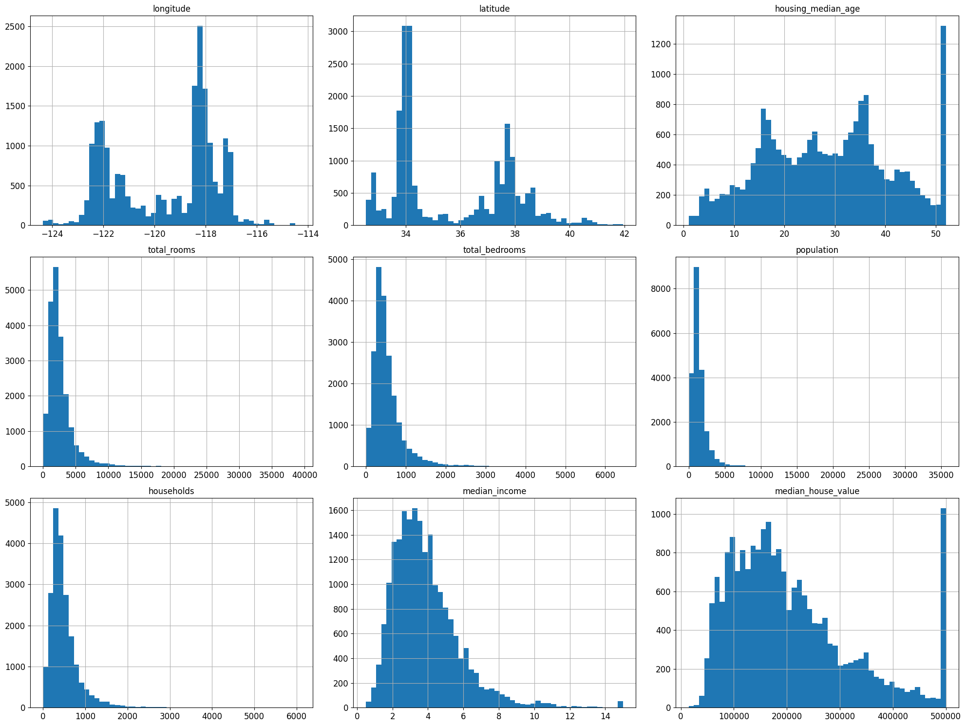
%matplotlib inline: 주피터 자체 백엔드를 사용하도록 지정 →IPython kernel 4.4.0, matplotlib 1.5.0이상부터는 자동으로 주피터 자체 백엔드로 설정- 몇가지 사항 확인
- 중간 소득(median income) 특성 US달러로 표현 X → 스케일 조정과 상한 15, 하한 3으로 조정(ex) 3은 실제로 30,000달러 의미)
- 중간 주택 연도(housing_median_age), 중간 주택 가격(median_house_value)의 최대,최소값도 한정 → 중간 주택 가격은 타켓 변수로 두가지 선택 방법이 필요
- 한계값 밖의 구역에 대한 정확한 레이블 구함
- 훈련 세트에서 이런 구역 제거($500,000가 넘는 값에 대한 예측은 평가 결과가 나쁘다고 보고 테스트 세트에서도 제거)
- 특성들의 스케일이 서로 많이 다르다
- 많은 히스토그램들의 꼬리가 두껍다 → 나중에 종 모양의 분포로 변형 필요
CAUTION
데이터를 깊게 들여다가 보기 전에 테스트 세트를 따로 두고 절대 참고하면 안됨
2.3.4 테스트 세트 만들기
- 데이터 스누핑 편향(data snooping): 테스트 세트로 파악한 패턴에 맞는 머신러닝 모델을 선택하여 기대한 성능이 나오지 않는 것
# 노트북의 실행 결과가 동일하도록
np.random.seed(42)
import numpy as np

# 예시로 만든 것입니다. 실전에서는 사이킷런의 train_test_split()를 사용하세요.
def split_train_test(data,test_ratio):
    shuffle_indices=np.random.permutation(len(data))
    test_set_size=int(len(data)*test_ratio)
    test_indices=shuffle_indices[:test_set_size]
    train_indices=shuffle_indices[test_set_size:]
    return data.iloc[train_indices],data.iloc[test_indices]
train_set,test_set=split_train_test(housing,0.2)
len(train_set)
16512
len(test_set)
4128
from zlib import crc32

def test_set_check(identifier, test_ratio):
    return crc32(np.int64(identifier) & 0xffffffff < test_ratio * 2**32)

def split_train_test_by_id(data,test_ratio,id_column):
    ids=data[id_column]
    in_test_set=ids.apply(lambda id_: test_set_check(id_,test_ratio))
    return data.loc[-in_test_set],data.loc[in_test_set]
위의 test_set_check() 함수가 파이썬 2와 파이썬 3에서 모두 잘 동작합니다. 초판에서는 모든 해시 함수를 지원하는 다음 방식을 제안했지만 느리고 파이썬 2를 지원하지 않습니다.
import hashlib

def test_set_check(identifier, test_ratio, hash=hashlib.md5):
    return hash(np.int64(identifier)).digest()[-1] < 256 * test_ratio
모든 해시 함수를 지원하고 파이썬 2와 파이썬 3에서 사용할 수 있는 함수를 원한다면 다음을 사용하세요.
def test_set_check(identifier, test_ratio, hash=hashlib.md5):
    return bytearray(hash(np.int64(identifier)).digest())[-1] < 256 * test_ratio
housing_with_id = housing.reset_index()   # `index` 열이 추가된 데이터프레임을 반환합니다
train_set, test_set = split_train_test_by_id(housing_with_id, 0.2, "index")
housing_with_id["id"] = housing["longitude"] * 1000 + housing["latitude"]
train_set, test_set = split_train_test_by_id(housing_with_id, 0.2, "id")
test_set.head()
| index | longitude | latitude | housing_median_age | total_rooms | total_bedrooms | population | households | median_income | median_house_value | ocean_proximity | id | |
|---|---|---|---|---|---|---|---|---|---|---|---|---|
| 8 | 8 | -122.26 | 37.84 | 42.0 | 2555.0 | 665.0 | 1206.0 | 595.0 | 2.0804 | 226700.0 | NEAR BAY | -122222.16 |
| 10 | 10 | -122.26 | 37.85 | 52.0 | 2202.0 | 434.0 | 910.0 | 402.0 | 3.2031 | 281500.0 | NEAR BAY | -122222.15 |
| 11 | 11 | -122.26 | 37.85 | 52.0 | 3503.0 | 752.0 | 1504.0 | 734.0 | 3.2705 | 241800.0 | NEAR BAY | -122222.15 |
| 12 | 12 | -122.26 | 37.85 | 52.0 | 2491.0 | 474.0 | 1098.0 | 468.0 | 3.0750 | 213500.0 | NEAR BAY | -122222.15 |
| 13 | 13 | -122.26 | 37.84 | 52.0 | 696.0 | 191.0 | 345.0 | 174.0 | 2.6736 | 191300.0 | NEAR BAY | -122222.16 |
- 무작위 샘플링
- 사이킷런의
train_test_splitrandom_state: 난수 초깃값 지정 매개변수- 행의 개수가 같은 여러 개의 데이터 셋을 넘겨서 인덱스 기반으로 나눌 수 있다. (데이터 프레임이 레이블에 따라 여러 개로 나누어져 있을 때 매우 유용)
- 사이킷런의
from sklearn.model_selection import train_test_split

train_set, test_set=train_test_split(housing,test_size=0.2, random_state=42)
test_set.head()
| longitude | latitude | housing_median_age | total_rooms | total_bedrooms | population | households | median_income | median_house_value | ocean_proximity | |
|---|---|---|---|---|---|---|---|---|---|---|
| 20046 | -119.01 | 36.06 | 25.0 | 1505.0 | NaN | 1392.0 | 359.0 | 1.6812 | 47700.0 | INLAND |
| 3024 | -119.46 | 35.14 | 30.0 | 2943.0 | NaN | 1565.0 | 584.0 | 2.5313 | 45800.0 | INLAND |
| 15663 | -122.44 | 37.80 | 52.0 | 3830.0 | NaN | 1310.0 | 963.0 | 3.4801 | 500001.0 | NEAR BAY |
| 20484 | -118.72 | 34.28 | 17.0 | 3051.0 | NaN | 1705.0 | 495.0 | 5.7376 | 218600.0 | <1H OCEAN |
| 9814 | -121.93 | 36.62 | 34.0 | 2351.0 | NaN | 1063.0 | 428.0 | 3.7250 | 278000.0 | NEAR OCEAN |
- 계층적 샘플링: 계층이라는 동질의 그룹으로 나뉘고 테스트 세트가 전체를 대표하도록 그룹 별로 올바른 수의 샘플을 추출
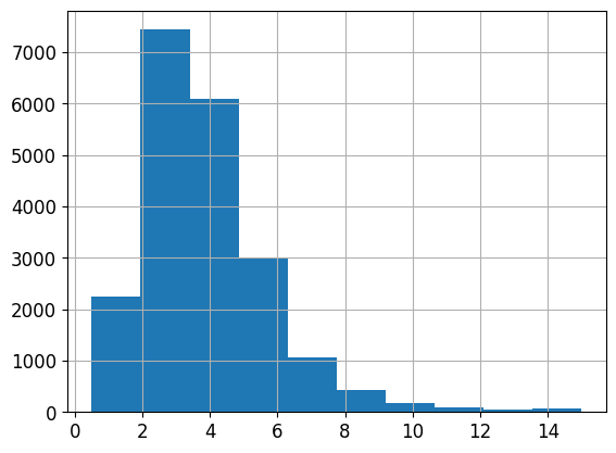
- 중간 소득이 중간 주택 가격 예측의 중요 변수라고 가정
- 소득에 대한 카테고리 특성 생성
housing['median_income'].hist()
<AxesSubplot:>
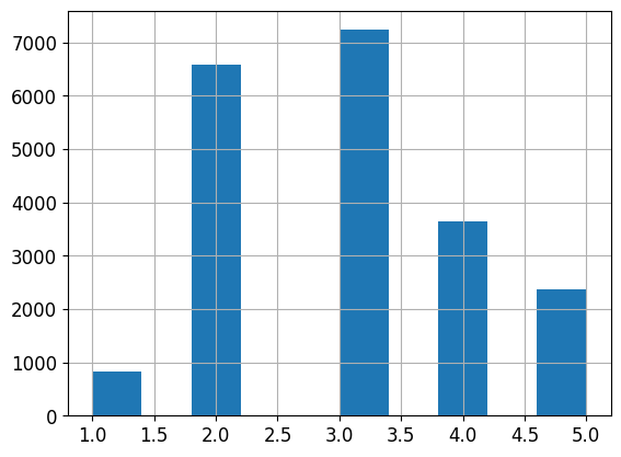
housing['income_cat']=pd.cut(housing['median_income'],
                            bins=[0.,1.5,3.0,4.5,6.,np.inf],
                            labels=[1,2,3,4,5])
housing['income_cat'].value_counts()
3    7236
2    6581
4    3639
5    2362
1     822
Name: income_cat, dtype: int64
housing['income_cat'].hist()
<AxesSubplot:>
- 사이킷런의
StratifiedShuffleSplit을 사용하여 소득 카테고리 기반으로 계층 샘플링 StratifiedShuffleSplitStratifiedKFold의 계층 샘플링과ShuffleSplit의 랜덤 샘플링을 합친 것- 매개변수
test_size+train_size의 합을 1이하로 지정 가능
from sklearn.model_selection import StratifiedShuffleSplit

split=StratifiedShuffleSplit(n_splits=1, test_size=0.2, random_state=42)
for train_index,test_index in split.split(housing,housing['income_cat']):
    strat_train_set=housing.loc[train_index]
    strat_test_set=housing.loc[test_index]
strat_test_set['income_cat'].value_counts()/len(strat_test_set)
3    0.350533
2    0.318798
4    0.176357
5    0.114341
1    0.039971
Name: income_cat, dtype: float64
housing['income_cat'].value_counts()/len(housing)
3    0.350581
2    0.318847
4    0.176308
5    0.114438
1    0.039826
Name: income_cat, dtype: float64
- 계층 샘플링의 경우 전체 데이터셋의 소득 카테고리 비율과 거의 유사
- 일반 무작위 샘플링은 많이 다르다
def income_cat_proportions(data):
    return data['income_cat'].value_counts()/len(data)

train_set, test_set=train_test_split(housing,test_size=0.2,random_state=42)

compare_props=pd.DataFrame({
    "Overall": income_cat_proportions(housing),
    "Stratified": income_cat_proportions(strat_test_set),
    "Random": income_cat_proportions(test_set),
}).sort_index()
compare_props["Rand. %error"]=100 * compare_props["Random"] / compare_props["Overall"] - 100
compare_props["Strat. %error"] = 100 * compare_props["Stratified"] / compare_props["Overall"] - 100
compare_props
| Overall | Stratified | Random | Rand. %error | Strat. %error | |
|---|---|---|---|---|---|
| 1 | 0.039826 | 0.039971 | 0.040213 | 0.973236 | 0.364964 |
| 2 | 0.318847 | 0.318798 | 0.324370 | 1.732260 | -0.015195 |
| 3 | 0.350581 | 0.350533 | 0.358527 | 2.266446 | -0.013820 |
| 4 | 0.176308 | 0.176357 | 0.167393 | -5.056334 | 0.027480 |
| 5 | 0.114438 | 0.114341 | 0.109496 | -4.318374 | -0.084674 |
- 판다스 데이터프레임
drop메서드axis0: 행 삭제, 1: 열 삭제inplace = True설정 시 호출된 객체에 새로운 데이터프레임 재할당하고 아무런 값도 반환 X
for set_ in (strat_train_set,strat_test_set):
    set_.drop("income_cat", axis=1,inplace=True)
2.4 데이터 이해를 위한 탐색과 시각화
- 훈련 세트에 대해서만 탐색
- 훈련 세트의 크기가 매우 크면 별도로 샘플링할 수도 있음
- 복사본 만들어 탐색
housing = strat_train_set.copy()
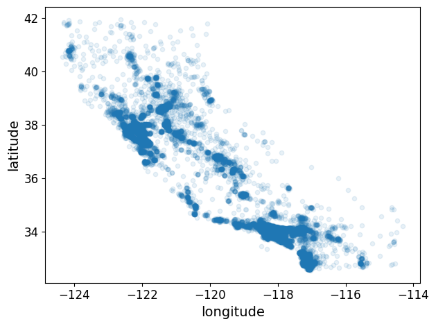
2.4.1 지리적 데이터 시각화
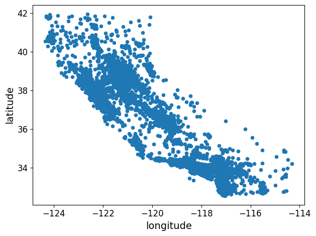
housing.plot(kind="scatter", x="longitude", y="latitude")
save_fig("bad_visualization_plot")
그림 저장: bad_visualization_plot
housing.plot(kind="scatter", x="longitude", y="latitude", alpha=0.1)
save_fig("better_visualization_plot")
그림 저장: better_visualization_plot
sharex=False 매개변수는 x-축의 값과 범례를 표시하지 못하는 버그를 수정합니다. 이는 임시 방편입니다(https://github.com/pandas-dev/pandas/issues/10611 참조). 수정 사항을 알려준 Wilmer Arellano에게 감사합니다.
housing.plot(kind="scatter", x="longitude", y="latitude", alpha=0.4,
            s=housing["population"]/100, label="population",figsize=(10,7),
            c="median_house_value", cmap=plt.get_cmap("jet"), colorbar=True,
            sharex=False)
plt.legend()
save_fig("housing_prices_scatterplot")
그림 저장: housing_prices_scatterplot
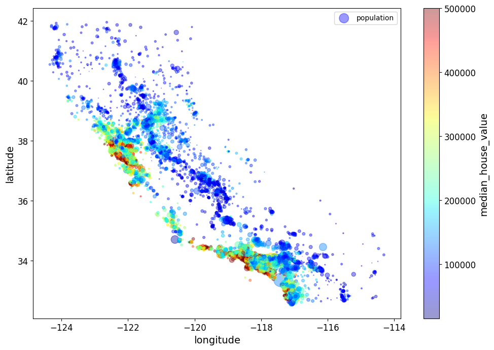
주택 가격은 지역과 인구 밀집에 관련이 매우 크다.
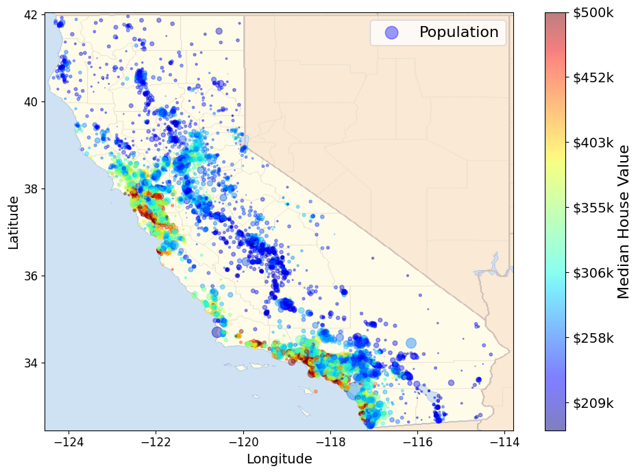
# Download the California image
images_path=os.path.join(PROJECT_ROOT_DIR,"images","end_to_end_project")
os.makedirs(images_path,exist_ok=True)
DOWNLOAD_ROOT="https://raw.githubusercontent.com/ageron/handson-ml2/master/"
filename="california.png"
print("Downloading",filename)
url=DOWNLOAD_ROOT+"images/end_to_end_project/" + filename
urllib.request.urlretrieve(url, os.path.join(images_path,filename))
Downloading california.png


('.\\images\\end_to_end_project\\california.png',
 <http.client.HTTPMessage at 0x1af7990e508>)
import matplotlib.image as mpimg
california_img=mpimg.imread(os.path.join(images_path,filename))
ax=housing.plot(kind="scatter", x="longitude", y="latitude", alpha=0.4,
            s=housing["population"]/100, label="Population",figsize=(10,7),
            c="median_house_value", cmap=plt.get_cmap("jet"), colorbar=False)
plt.imshow(california_img,extent=[-124.55, -113.80, 32.45, 42.05],alpha=0.5,
          cmap=plt.get_cmap("jet"))
plt.ylabel("Latitude", fontsize=14)
plt.xlabel("Longitude", fontsize=14)

prices=housing["median_house_value"]
tick_values=np.linspace(prices.min(),prices.max(), 11)
cbar=plt.colorbar(ticks=tick_values/prices.max())
cbar.ax.set_yticklabels(["$%dk"%(round(v/1000)) for v in tick_values], fontsize=14)
cbar.set_label("Median House Value", fontsize=16)

plt.legend(fontsize=16)
save_fig("california_housing_prices_plot")
plt.show()
그림 저장: california_housing_prices_plot
2.4.2 상관관계 조사
corr_matrix = housing.corr()
corr_matrix["median_house_value"].sort_values(ascending=False)
median_house_value    1.000000
median_income         0.687151
total_rooms           0.135140
housing_median_age    0.114146
households            0.064590
total_bedrooms        0.047781
population           -0.026882
longitude            -0.047466
latitude             -0.142673
Name: median_house_value, dtype: float64
- 상관 계수
- 선형적인 상관관계만 측정(비선형적 관계 알 수 없다)
- 상관계수 수치와 기울기는 관련성이 없다
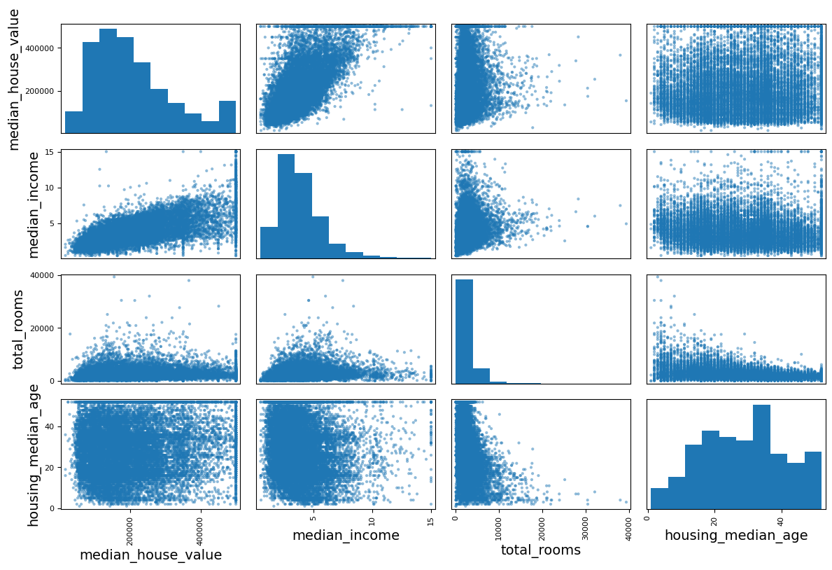
from pandas.plotting import scatter_matrix

attributes=["median_house_value","median_income","total_rooms","housing_median_age"]
scatter_matrix(housing[attributes],figsize=(12,8))
save_fig("scatter_matrix_plot")
그림 저장: scatter_matrix_plot
housing.plot(kind="scatter", x="median_income", y="median_house_value", alpha=0.1)
plt.axis([0,16,0,550000])
save_fig("income_vs_house_value_scatterplot")
그림 저장: income_vs_house_value_scatterplot
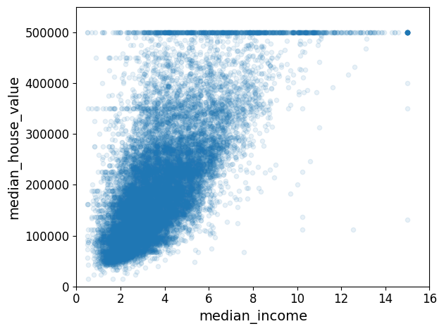
- 중간 주택 가격(median_house_value)와 중간 소득(median income)의 상과관계 산점도
- 상관관계 매우 강함
- 앞서 본
$500,000 과$450,000,$350,000,$280,000에서 수평선의 분포 보임 → 이런 이상한 형태를 학습하지 않도록 해당 구역을 제거하는 것이 좋다.
2.4.3 특성 조합으로 실험
housing["rooms_per_household"]=housing["total_rooms"]/housing["households"]
housing["bedrooms_per_room"]=housing["total_bedrooms"]/housing["total_rooms"]
housing["population_per_household"]=housing["population"]/housing["households"]
- 가구당 방 개수, 침실/방, 가구당 인원 등의 유용해 보이는 특성 생성
corr_matrix=housing.corr()
corr_matrix["median_house_value"].sort_values(ascending=False)
median_house_value          1.000000
median_income               0.687151
rooms_per_household         0.146255
total_rooms                 0.135140
housing_median_age          0.114146
households                  0.064590
total_bedrooms              0.047781
population_per_household   -0.021991
population                 -0.026882
longitude                  -0.047466
latitude                   -0.142673
bedrooms_per_room          -0.259952
Name: median_house_value, dtype: float64
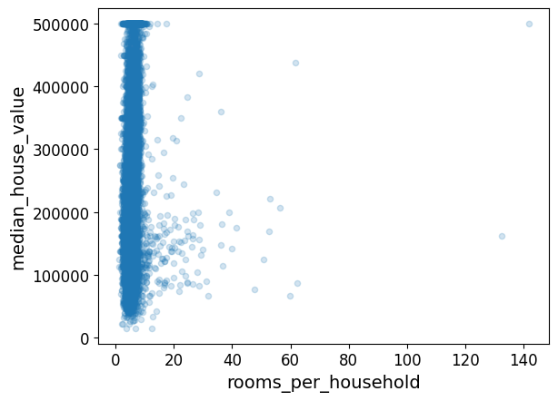
housing.plot(kind="scatter",x="rooms_per_household",y="median_house_value",alpha=0.2)
plt.show()
housing.describe()
| longitude | latitude | housing_median_age | total_rooms | total_bedrooms | population | households | median_income | median_house_value | rooms_per_household | bedrooms_per_room | population_per_household | |
|---|---|---|---|---|---|---|---|---|---|---|---|---|
| count | 16512.000000 | 16512.000000 | 16512.000000 | 16512.000000 | 16354.000000 | 16512.000000 | 16512.000000 | 16512.000000 | 16512.000000 | 16512.000000 | 16354.000000 | 16512.000000 |
| mean | -119.575635 | 35.639314 | 28.653404 | 2622.539789 | 534.914639 | 1419.687379 | 497.011810 | 3.875884 | 207005.322372 | 5.440406 | 0.212873 | 3.096469 |
| std | 2.001828 | 2.137963 | 12.574819 | 2138.417080 | 412.665649 | 1115.663036 | 375.696156 | 1.904931 | 115701.297250 | 2.611696 | 0.057378 | 11.584825 |
| min | -124.350000 | 32.540000 | 1.000000 | 6.000000 | 2.000000 | 3.000000 | 2.000000 | 0.499900 | 14999.000000 | 1.130435 | 0.100000 | 0.692308 |
| 25% | -121.800000 | 33.940000 | 18.000000 | 1443.000000 | 295.000000 | 784.000000 | 279.000000 | 2.566950 | 119800.000000 | 4.442168 | 0.175304 | 2.431352 |
| 50% | -118.510000 | 34.260000 | 29.000000 | 2119.000000 | 433.000000 | 1164.000000 | 408.000000 | 3.541550 | 179500.000000 | 5.232342 | 0.203027 | 2.817661 |
| 75% | -118.010000 | 37.720000 | 37.000000 | 3141.000000 | 644.000000 | 1719.000000 | 602.000000 | 4.745325 | 263900.000000 | 6.056361 | 0.239816 | 3.281420 |
| max | -114.310000 | 41.950000 | 52.000000 | 39320.000000 | 6210.000000 | 35682.000000 | 5358.000000 | 15.000100 | 500001.000000 | 141.909091 | 1.000000 | 1243.333333 |
- 침실/방, 가구당 방 개수 특성들은 기존의 특성들보다 중간 주택 가격과의 상관관계가 높다.
- 특히 머신러닝 프로젝트에서는 빠른 프로토 타이핑과 반복적인 프로세스가 권장됨
2.5 머신러닝 알고리즘을 위한 데이터 준비
- 이 작업을 수동으로 하는 대신 자동화 함수를 생성해야하는 이유
- 어떤 데이터 셋에 대해서도 데이터 변환을 쉽게 반복 가능 (ex: 다음번에 새로운 데이터셋 사용할 때)
- 향후 프로젝트에 사용 가능한 변환 라이브러리 점진적 구축
- 실제 시스템에서 알고리즘에 새 데이터 주입 전 변환 시 사용 가능
- 여러가지 데이터 변화 쉽게 시도 가능하고, 어떤 조합이 가장 좋은지 확인하는데 편리
- 예측 변수, 레이블 분리
housing=strat_train_set.drop("median_house_value",axis=1)# 훈련 세트를 위해 레이블 제거
housing_labels=strat_train_set["median_house_value"].copy()
drop()은 데이터 복사본을 만들어 strat_train_set에 영향을 주지 않음
2.5.1 데이터 정제
- 누락된 값 처리
housing.dropna(subset=["total_bedrooms"])    # 옵션 1
housing.drop("total_bedrooms", axis=1)       # 옵션 2
median = housing["total_bedrooms"].median()  # 옵션 3
housing["total_bedrooms"].fillna(median, inplace=True)
- 각 옵션을 설명하기 위해 주택 데이터셋의 복사본을 만듭니다. 이 때 적어도 하나의 열이 비어 있는 행만 고릅니다. 이렇게 하면 각 옵션의 정확한 동작을 눈으로 쉽게 확인할 수 있습니다.
sample_incomplete_rows=housing[housing.isnull().any(axis=1)].head()
sample_incomplete_rows
| longitude | latitude | housing_median_age | total_rooms | total_bedrooms | population | households | median_income | ocean_proximity | |
|---|---|---|---|---|---|---|---|---|---|
| 1606 | -122.08 | 37.88 | 26.0 | 2947.0 | NaN | 825.0 | 626.0 | 2.9330 | NEAR BAY |
| 10915 | -117.87 | 33.73 | 45.0 | 2264.0 | NaN | 1970.0 | 499.0 | 3.4193 | <1H OCEAN |
| 19150 | -122.70 | 38.35 | 14.0 | 2313.0 | NaN | 954.0 | 397.0 | 3.7813 | <1H OCEAN |
| 4186 | -118.23 | 34.13 | 48.0 | 1308.0 | NaN | 835.0 | 294.0 | 4.2891 | <1H OCEAN |
| 16885 | -122.40 | 37.58 | 26.0 | 3281.0 | NaN | 1145.0 | 480.0 | 6.3580 | NEAR OCEAN |
sample_incomplete_rows.dropna(subset=["total_bedrooms"]) # 옵션 1
| longitude | latitude | housing_median_age | total_rooms | total_bedrooms | population | households | median_income | ocean_proximity |
|---|
sample_incomplete_rows.drop("total_bedrooms",axis=1) # 옵션 2
| longitude | latitude | housing_median_age | total_rooms | population | households | median_income | ocean_proximity | |
|---|---|---|---|---|---|---|---|---|
| 1606 | -122.08 | 37.88 | 26.0 | 2947.0 | 825.0 | 626.0 | 2.9330 | NEAR BAY |
| 10915 | -117.87 | 33.73 | 45.0 | 2264.0 | 1970.0 | 499.0 | 3.4193 | <1H OCEAN |
| 19150 | -122.70 | 38.35 | 14.0 | 2313.0 | 954.0 | 397.0 | 3.7813 | <1H OCEAN |
| 4186 | -118.23 | 34.13 | 48.0 | 1308.0 | 835.0 | 294.0 | 4.2891 | <1H OCEAN |
| 16885 | -122.40 | 37.58 | 26.0 | 3281.0 | 1145.0 | 480.0 | 6.3580 | NEAR OCEAN |
median = housing["total_bedrooms"].median()
sample_incomplete_rows["total_bedrooms"].fillna(median, inplace=True) # 옵션 3
sample_incomplete_rows
| longitude | latitude | housing_median_age | total_rooms | total_bedrooms | population | households | median_income | ocean_proximity | |
|---|---|---|---|---|---|---|---|---|---|
| 1606 | -122.08 | 37.88 | 26.0 | 2947.0 | 433.0 | 825.0 | 626.0 | 2.9330 | NEAR BAY |
| 10915 | -117.87 | 33.73 | 45.0 | 2264.0 | 433.0 | 1970.0 | 499.0 | 3.4193 | <1H OCEAN |
| 19150 | -122.70 | 38.35 | 14.0 | 2313.0 | 433.0 | 954.0 | 397.0 | 3.7813 | <1H OCEAN |
| 4186 | -118.23 | 34.13 | 48.0 | 1308.0 | 433.0 | 835.0 | 294.0 | 4.2891 | <1H OCEAN |
| 16885 | -122.40 | 37.58 | 26.0 | 3281.0 | 433.0 | 1145.0 | 480.0 | 6.3580 | NEAR OCEAN |
from sklearn.impute import SimpleImputer
imputer=SimpleImputer(strategy="median")
중간값이 수치형 특성에서만 계산될 수 있기 때문에 텍스트 특성을 삭제합니다:
housing_num=housing.drop("ocean_proximity",axis=1)
imputer.fit(housing_num)
SimpleImputer(strategy='median')
imputer.statistics_ # 각 특성의 중간값
array([-118.51   ,   34.26   ,   29.     , 2119.     ,  433.     ,
       1164.     ,  408.     ,    3.54155])
각 특성의 중간 값이 수동으로 계산한 것과 같은지 확인해 보세요:
housing_num.median().values
array([-118.51   ,   34.26   ,   29.     , 2119.     ,  433.     ,
       1164.     ,  408.     ,    3.54155])
X=imputer.transform(housing_num)
housing_tr=pd.DataFrame(X,columns=housing_num.columns,
                       index=housing_num.index)
housing_tr.loc[sample_incomplete_rows.index.values]
| longitude | latitude | housing_median_age | total_rooms | total_bedrooms | population | households | median_income | |
|---|---|---|---|---|---|---|---|---|
| 1606 | -122.08 | 37.88 | 26.0 | 2947.0 | 433.0 | 825.0 | 626.0 | 2.9330 |
| 10915 | -117.87 | 33.73 | 45.0 | 2264.0 | 433.0 | 1970.0 | 499.0 | 3.4193 |
| 19150 | -122.70 | 38.35 | 14.0 | 2313.0 | 433.0 | 954.0 | 397.0 | 3.7813 |
| 4186 | -118.23 | 34.13 | 48.0 | 1308.0 | 433.0 | 835.0 | 294.0 | 4.2891 |
| 16885 | -122.40 | 37.58 | 26.0 | 3281.0 | 433.0 | 1145.0 | 480.0 | 6.3580 |
imputer.strategy
'median'
housing_tr.head()
| longitude | latitude | housing_median_age | total_rooms | total_bedrooms | population | households | median_income | |
|---|---|---|---|---|---|---|---|---|
| 12655 | -121.46 | 38.52 | 29.0 | 3873.0 | 797.0 | 2237.0 | 706.0 | 2.1736 |
| 15502 | -117.23 | 33.09 | 7.0 | 5320.0 | 855.0 | 2015.0 | 768.0 | 6.3373 |
| 2908 | -119.04 | 35.37 | 44.0 | 1618.0 | 310.0 | 667.0 | 300.0 | 2.8750 |
| 14053 | -117.13 | 32.75 | 24.0 | 1877.0 | 519.0 | 898.0 | 483.0 | 2.2264 |
| 20496 | -118.70 | 34.28 | 27.0 | 3536.0 | 646.0 | 1837.0 | 580.0 | 4.4964 |
- 사이킷런의
SimpleImputer- 각 특성의 중간 값 계산해서 객체의
statistics속성에 저장 - 모든 수치형 특성에
imputer적용하는것이 바람직(새로운 데이터에서 어떤 값이 누락될지 모르기 때문)
- 각 특성의 중간 값 계산해서 객체의
- 사이킷런의 설계 철학
- 일관성: 모든 객체가 일관되고 단순한 인터페이스 공유
- 추정기(estimator)
- 데이터셋 기반으로 일련의 모델 파라미터들을 추정하는 객체 ex)
imputer fit()메서드에 의해 추정 수행되고 하나의 매개변수로 하나의 데이터셋만 전달(지도 학습: 매개변수 두개, 두번째 데이터셋은 레이블)
- 데이터셋 기반으로 일련의 모델 파라미터들을 추정하는 객체 ex)
- 변환기(transformer)
- (
imputer같이) 데이터셋을 변환하는 추정기 - 데이터셋을 매개변수로 전달받은
transform()메서드가 변환 수행 fit_transform:fit()과transform()을 연달아 호출하는 것과 동일
- (
- 예측기(predictor)
- 일부 추정기는 주어진 데이터셋에 대해 예측을 만들 수 있다 ex)
LinearRegression모델 → 예측기 predict(): 새로운 데이터셋을 받아 이에 상응하는 예측값을 반환score(): 테스트 세트를 사용해 예측의 품질을 측정함
- 일부 추정기는 주어진 데이터셋에 대해 예측을 만들 수 있다 ex)
- 추정기(estimator)
- 검사 가능
- 모든 추정기의 하이퍼파라미터는 공개 인스턴스 변수로 직접 접근 가능 ex)
imputer.strategy - 모든 추정기의 학습된 모델파라미터 접미사로 밑줄을 붙여서 공개 인스턴스 변수로 제공 ex)
imputer.statistics_
- 모든 추정기의 하이퍼파라미터는 공개 인스턴스 변수로 직접 접근 가능 ex)
- 클래스 남용 방지: 데이터셋을 넘파이 배열, 사이파이 희소 행렬로 표현
- 조합성: 기존의 구성요소 최대한 재사용 ex) 여러 변환기를 연결한 다음 마지막에 추정기 하나를 배치한
Pipeline추정기 - 합리적인 기본 값: 대부분의 매개변수에 합리적인 기본값 지정 → 일단 돌아가는 기본 시스템 빠르게 만들 수 있다.
- 일관성: 모든 객체가 일관되고 단순한 인터페이스 공유
2.5.2 텍스트와 범주형 특성 다루기
이제 범주형 입력 특성인 ocean_proximity을 전처리합니다:
housing_cat=housing[["ocean_proximity"]]
housing_cat.head(10)
| ocean_proximity | |
|---|---|
| 12655 | INLAND |
| 15502 | NEAR OCEAN |
| 2908 | INLAND |
| 14053 | NEAR OCEAN |
| 20496 | <1H OCEAN |
| 1481 | NEAR BAY |
| 18125 | <1H OCEAN |
| 5830 | <1H OCEAN |
| 17989 | <1H OCEAN |
| 4861 | <1H OCEAN |
OrdinalEncoder- 범주형 특성 값을 숫자로 변환
- 문제: 머신러닝 알고리즘이 가까운 값을 더 비슷하다고 생각
from sklearn.preprocessing import OrdinalEncoder

ordinal_encoder=OrdinalEncoder()
housing_cat_encoded=ordinal_encoder.fit_transform(housing_cat)
housing_cat_encoded[:10]
array([[1.],
       [4.],
       [1.],
       [4.],
       [0.],
       [3.],
       [0.],
       [0.],
       [0.],
       [0.]])
ordinal_encoder.categories_ # 카테고리 목록
[array(['<1H OCEAN', 'INLAND', 'ISLAND', 'NEAR BAY', 'NEAR OCEAN'],
       dtype=object)]
OneHotEncoder- 한 특성만 1, 나머지는 모두 0 (더미 특성: 새로운 특성)
- 사이파이 희소 행렬로 출력 →
numpy배열로 바꾸려면toarray()메서드 사용 - 0이 아닌 원소의 위치만 저장하므로 카테고리의 수가 많을 때 매우 효율적
from sklearn.preprocessing import OneHotEncoder

cat_encoder=OneHotEncoder()
housing_cat_1hot=cat_encoder.fit_transform(housing_cat)
housing_cat_1hot
<16512x5 sparse matrix of type '<class 'numpy.float64'>'
	with 16512 stored elements in Compressed Sparse Row format>
housing_cat_1hot.toarray()
array([[0., 1., 0., 0., 0.],
       [0., 0., 0., 0., 1.],
       [0., 1., 0., 0., 0.],
       ...,
       [1., 0., 0., 0., 0.],
       [1., 0., 0., 0., 0.],
       [0., 1., 0., 0., 0.]])
또는 OneHotEncoder를 만들 때 sparse=False로 지정할 수 있습니다:
cat_encoder=OneHotEncoder(sparse=False)
housing_cat_1hot=cat_encoder.fit_transform(housing_cat)
housing_cat_1hot
array([[0., 1., 0., 0., 0.],
       [0., 0., 0., 0., 1.],
       [0., 1., 0., 0., 0.],
       ...,
       [1., 0., 0., 0., 0.],
       [1., 0., 0., 0., 0.],
       [0., 1., 0., 0., 0.]])
cat_encoder.categories_
[array(['<1H OCEAN', 'INLAND', 'ISLAND', 'NEAR BAY', 'NEAR OCEAN'],
       dtype=object)]
OrdinalEncoder,OneHotEncoder둘다 인코더의categories_인스턴스 변수를 사용해 카테고리 리스트를 얻을 수 있다.
Tip
- 카테고리 특성이 많으면 원-핫 인코딩은 많은 수의 입력 특성 생성 → 훈련을 느리고 성능 감소
- 범주형 입력 값 이 특성과 관련된 숫자형 특성으로 변경 ex)
ocean proximity특성 해안까지의 거리로 변경- 각 카테고리 임베딩으로 변환(훈련동안 각 카테고리의 표현이 학습) → 표현학습의 한 예시
- 표현학습
- 각 카테고리를 임베딩으로 바꿔 훈련하는 동안 각 카테고리의 표현 학습
- 임베딩: 학습 가능한 저차원의 벡터로 변경한 결과 혹은 그 과정 전체
2.5.3 나만의 변환기
- 덕타이핑: 상속이나 인터페이스 구현이 아닌 객체의 속성이나 메서드가 객체의 유형을 결정하는 방식
- 사이킷런은 덕타이핑 지원 ->
fit(),transform(),fit_transform()메서드를 구현한 파이썬 클래스 만들면 됨 TransformerMixin상속하면fit_transform()자동 생성,BaseEstimator상속하면 하이퍼파라미터 튜닝에 필요한get_params(),set_params()메서드 얻음
앞서말한 조합 특성 추가 간단한 변환기
from sklearn.base import TransformerMixin, BaseEstimator

#열 인덱스
rooms_ix, bedrooms_ix, population_ix, households_ix=3,4,5,6

class CombinedAttributesAdder(TransformerMixin,BaseEstimator):
    def __init__(self, add_bedrooms_per_room=True): # *args 또는 **kargs 없음
        self.add_bedrooms_per_room=add_bedrooms_per_room
    def fit(self,X,y=None):
        return self # 아무것도 하지 않음
    def transform(self, X):
        rooms_per_household=X[:,rooms_ix]/X[:,households_ix]
        population_per_household=X[:,population_ix]/X[:,households_ix]
        if self.add_bedrooms_per_room:
            bedrooms_per_room=X[:,bedrooms_ix]/X[:,rooms_ix]
            return np.c_[X,rooms_per_household,population_per_household,bedrooms_per_room]
        else:
            return np.c_[X,rooms_per_household,population_per_household]

attr_adder=CombinedAttributesAdder(add_bedrooms_per_room=False)
housing_extra_attribs=attr_adder.transform(housing.to_numpy())
책에서는 간단하게 인덱스 (3, 4, 5, 6)을 하드코딩했지만 다음처럼 동적으로 처리하는 것이 더 좋습니다:
col_names="total_rooms","total_bedrooms","population","households"
rooms_ix, bedrooms_ix, population_ix, households_ix=[housing.columns.get_loc(c) for c in col_names]# 열 인덱스 구하기
또한 housing_extra_attribs는 넘파이 배열이기 때문에 열 이름이 없습니다(안타깝지만 사이킷런을 사용할 때 생기는 문제입니다). DataFrame으로 복원하려면 다음과 같이 할 수 있습니다:
housing_extra_attribs=pd.DataFrame(
        housing_extra_attribs,
        columns=list(housing.columns)+["rooms_per_household", "population_per_household"],
    index=housing.index)
housing_extra_attribs.head()
| longitude | latitude | housing_median_age | total_rooms | total_bedrooms | population | households | median_income | ocean_proximity | rooms_per_household | population_per_household | |
|---|---|---|---|---|---|---|---|---|---|---|---|
| 12655 | -121.46 | 38.52 | 29.0 | 3873.0 | 797.0 | 2237.0 | 706.0 | 2.1736 | INLAND | 5.485836 | 3.168555 |
| 15502 | -117.23 | 33.09 | 7.0 | 5320.0 | 855.0 | 2015.0 | 768.0 | 6.3373 | NEAR OCEAN | 6.927083 | 2.623698 |
| 2908 | -119.04 | 35.37 | 44.0 | 1618.0 | 310.0 | 667.0 | 300.0 | 2.875 | INLAND | 5.393333 | 2.223333 |
| 14053 | -117.13 | 32.75 | 24.0 | 1877.0 | 519.0 | 898.0 | 483.0 | 2.2264 | NEAR OCEAN | 3.886128 | 1.859213 |
| 20496 | -118.7 | 34.28 | 27.0 | 3536.0 | 646.0 | 1837.0 | 580.0 | 4.4964 | <1H OCEAN | 6.096552 | 3.167241 |
2.5.4 특성 스케일링
- 타깃값에 대한 스케일링 일반적으로 불필요
- min-max 스케일링(정규화로 많이 불림)
- x-min/max-min (0~1 범위로 값을 조정)
MinMaxScaler변환기 제공feature_range매개변수로 범위 변경 가능
- 표준화
- x-average/std (평균:0, 분산:1)
- 범위의 상한과 하한이 없어 문제가 될 수 있다. ex) 인공신경망은 입력값의 기대값이 0~1사이
- 이상치에 영향을 덜 받음
StandardScaler변환기 제공
CAUTION
훈련데이터에 대해서만fit()한 후, 훈련 데이터 와 테스트 데이터에 대해transform()메서드 사용
2.5.5 변환 파이프라인
Pipeline- 연속된 단계를 나타내는 이름/추정기 쌍을 입력받음
- 마지막 단계는 변환기와 추정기 모두 사용 가능 (나머지는 변환기) → 즉, (
fit+transform) orfit_transform가져야함
from sklearn.pipeline import Pipeline
from sklearn.preprocessing import StandardScaler

num_pipeline=Pipeline([
    ('imputer', SimpleImputer(strategy="median")),
    ('attribs_adder', CombinedAttributesAdder()),
    ('std_scaler', StandardScaler()),
])

housing_tr=num_pipeline.fit_transform(housing_num)
housing_tr
array([[-0.94135046,  1.34743822,  0.02756357, ...,  0.01739526,
         0.00622264, -0.12112176],
       [ 1.17178212, -1.19243966, -1.72201763, ...,  0.56925554,
        -0.04081077, -0.81086696],
       [ 0.26758118, -0.1259716 ,  1.22045984, ..., -0.01802432,
        -0.07537122, -0.33827252],
       ...,
       [-1.5707942 ,  1.31001828,  1.53856552, ..., -0.5092404 ,
        -0.03743619,  0.32286937],
       [-1.56080303,  1.2492109 , -1.1653327 , ...,  0.32814891,
        -0.05915604, -0.45702273],
       [-1.28105026,  2.02567448, -0.13148926, ...,  0.01407228,
         0.00657083, -0.12169672]])
ColumnTransformer- 하나의 변환기로 각 열마다 적절한 변환을 적용하여 모든 열을 처리
- 단계
- 수치형, 범주형 열 이름의 리스트 생성
ColumnTransformer객체에 이름, 변환기, 변환기가 적용될 열 이름(또는 인덱스) 튜플의 리스트 입력- 각 변환기를 적절한 열에 적용(반환하는 행의 개수 같아야함)
OneHotEncoder는 희소 행렬,num_pipeline은 밀집 행렬 반환 → 최종 행렬 밀집도 임계값 기준으로 결과 반환(기본적으로sparse_threshold=0.3)- 여기서는 밀집 행렬 반환
TIP
drop: 삭제하는 열,passthrough: 변환을 적용하지 않을 열- 나열되지 않은 열을 기본적으로 삭제
from sklearn.compose import ColumnTransformer

num_attribs=list(housing_num)
cat_attribs=["ocean_proximity"]

full_pipeline=ColumnTransformer([
    ("num", num_pipeline, num_attribs),
    ("cat", OneHotEncoder(), cat_attribs),
])

housing_prepared=full_pipeline.fit_transform(housing)
housing_prepared
array([[-0.94135046,  1.34743822,  0.02756357, ...,  0.        ,
         0.        ,  0.        ],
       [ 1.17178212, -1.19243966, -1.72201763, ...,  0.        ,
         0.        ,  1.        ],
       [ 0.26758118, -0.1259716 ,  1.22045984, ...,  0.        ,
         0.        ,  0.        ],
       ...,
       [-1.5707942 ,  1.31001828,  1.53856552, ...,  0.        ,
         0.        ,  0.        ],
       [-1.56080303,  1.2492109 , -1.1653327 , ...,  0.        ,
         0.        ,  0.        ],
       [-1.28105026,  2.02567448, -0.13148926, ...,  0.        ,
         0.        ,  0.        ]])
housing_prepared.shape
(16512, 16)
다음은 (판다스 DataFrame 열의 일부를 선택하기 위해) DataFrameSelector 변환기와 FeatureUnion를 사용한 예전 방식입니다:
from sklearn.base import BaseEstimator, TransformerMixin

# 수치형 열과 범주형 열을 선택하기 위한 클래스
class OldDataFrameSelector(BaseEstimator, TransformerMixin):
    def __init__(self, attribute_names):
        self.attribute_names = attribute_names
    def fit(self, X, y=None):
        return self
    def transform(self, X):
        return X[self.attribute_names].values
하나의 큰 파이프라인에 이들을 모두 결합하여 수치형과 범주형 특성을 전처리합니다:
num_attribs = list(housing_num)
cat_attribs = ["ocean_proximity"]

old_num_pipeline = Pipeline([
        ('selector', OldDataFrameSelector(num_attribs)),
        ('imputer', SimpleImputer(strategy="median")),
        ('attribs_adder', CombinedAttributesAdder()),
        ('std_scaler', StandardScaler()),
    ])

old_cat_pipeline = Pipeline([
        ('selector', OldDataFrameSelector(cat_attribs)),
        ('cat_encoder', OneHotEncoder(sparse=False)),
    ])
from sklearn.pipeline import FeatureUnion

old_full_pipeline = FeatureUnion(transformer_list=[
        ("num_pipeline", old_num_pipeline),
        ("cat_pipeline", old_cat_pipeline),
    ])
old_housing_prepared = old_full_pipeline.fit_transform(housing)
old_housing_prepared
array([[-0.94135046,  1.34743822,  0.02756357, ...,  0.        ,
         0.        ,  0.        ],
       [ 1.17178212, -1.19243966, -1.72201763, ...,  0.        ,
         0.        ,  1.        ],
       [ 0.26758118, -0.1259716 ,  1.22045984, ...,  0.        ,
         0.        ,  0.        ],
       ...,
       [-1.5707942 ,  1.31001828,  1.53856552, ...,  0.        ,
         0.        ,  0.        ],
       [-1.56080303,  1.2492109 , -1.1653327 , ...,  0.        ,
         0.        ,  0.        ],
       [-1.28105026,  2.02567448, -0.13148926, ...,  0.        ,
         0.        ,  0.        ]])
ColumnTransformer의 결과와 동일합니다:
np.allclose(housing_prepared, old_housing_prepared)
True
2.6 모델 선택과 훈련
2.6.1 훈련 세트에서 훈련하고 평가하기
from sklearn.linear_model import LinearRegression

lin_reg=LinearRegression()
lin_reg.fit(housing_prepared,housing_labels)
LinearRegression()
# 훈련 샘플 몇 개를 사용해 전체 파이프라인을 적용해 보겠습니다
some_data=housing.iloc[:5]
some_labels=housing_labels.iloc[:5]
some_data_prepared=full_pipeline.transform(some_data)

print("예측: ", lin_reg.predict(some_data_prepared))
예측:  [ 85657.90192014 305492.60737488 152056.46122456 186095.70946094
 244550.67966089]
실제 값과 비교
print("레이블: ", list(some_labels))
레이블: [72100.0, 279600.0, 82700.0, 112500.0, 238300.0]
some_data_prepared
array([[-0.94135046,  1.34743822,  0.02756357,  0.58477745,  0.64037127,
         0.73260236,  0.55628602, -0.8936472 ,  0.01739526,  0.00622264,
        -0.12112176,  0.        ,  1.        ,  0.        ,  0.        ,
         0.        ],
       [ 1.17178212, -1.19243966, -1.72201763,  1.26146668,  0.78156132,
         0.53361152,  0.72131799,  1.292168  ,  0.56925554, -0.04081077,
        -0.81086696,  0.        ,  0.        ,  0.        ,  0.        ,
         1.        ],
       [ 0.26758118, -0.1259716 ,  1.22045984, -0.46977281, -0.54513828,
        -0.67467519, -0.52440722, -0.52543365, -0.01802432, -0.07537122,
        -0.33827252,  0.        ,  1.        ,  0.        ,  0.        ,
         0.        ],
       [ 1.22173797, -1.35147437, -0.37006852, -0.34865152, -0.03636724,
        -0.46761716, -0.03729672, -0.86592882, -0.59513997, -0.10680295,
         0.96120521,  0.        ,  0.        ,  0.        ,  0.        ,
         1.        ],
       [ 0.43743108, -0.63581817, -0.13148926,  0.42717947,  0.27279028,
         0.37406031,  0.22089846,  0.32575178,  0.2512412 ,  0.00610923,
        -0.47451338,  1.        ,  0.        ,  0.        ,  0.        ,
         0.        ]])
from sklearn.metrics import mean_squared_error

housing_predictions=lin_reg.predict(housing_prepared)
lin_mse=mean_squared_error(housing_labels,housing_predictions)
lin_rmse=np.sqrt(lin_mse)
lin_rmse
68627.87390018745
노트: 사이킷런 0.22 버전부터는 squared=False 매개변수로 mean_squared_error() 함수를 호출하면 RMSE를 바로 얻을 수 있습니다.
from sklearn.metrics import mean_absolute_error

lin_mae = mean_absolute_error(housing_labels, housing_predictions)
lin_mae
49438.66860915801
- 선형 회귀 모델 → 과소적합
- 더 복잡한 모델, 더 좋은 특성 주입
- 더 복잡한 모델 선택 →
DecisionTreeRegressor
from sklearn.tree import DecisionTreeRegressor

tree_reg = DecisionTreeRegressor(random_state=42)
tree_reg.fit(housing_prepared, housing_labels)
DecisionTreeRegressor(random_state=42)
housing_predictions = tree_reg.predict(housing_prepared)
tree_mse = mean_squared_error(housing_labels, housing_predictions)
tree_rmse = np.sqrt(tree_mse)
tree_rmse
0.0
- 결정 트리 → 과대적합
- 훈련 세트의 일부분으로 훈련하고 다른 일부분은 검증으로 사용해야함
2.6.2 교차 검증을 사용한 평가
- k-fold cross-validation
- 훈련 세트를 k개의 폴드(fold)로 분할하여 매번 다른 폴드를 평가에 사용 (k번 훈련하고 평가)
- 사이킷런 교차검증 기능
scoring매개변수에 효용함수 기대(클수록 좋은) → 그래서neg_mean_squared_error,-scores사용
from sklearn.model_selection import cross_val_score

scores = cross_val_score(tree_reg, housing_prepared, housing_labels,
                         scoring="neg_mean_squared_error", cv=10)
tree_rmse_scores = np.sqrt(-scores)
def display_scores(scores):
    print("점수:", scores)
    print("평균:", scores.mean())
    print("표준 편차:", scores.std())

display_scores(tree_rmse_scores)
점수: [72831.45749112 69973.18438322 69528.56551415 72517.78229792
 69145.50006909 79094.74123727 68960.045444   73344.50225684
 69826.02473916 71077.09753998]
평균: 71629.89009727491
표준 편차: 2914.035468468928
lin_scores = cross_val_score(lin_reg, housing_prepared, housing_labels,
                             scoring="neg_mean_squared_error", cv=10)
lin_rmse_scores = np.sqrt(-lin_scores)
display_scores(lin_rmse_scores)
점수: [71762.76364394 64114.99166359 67771.17124356 68635.19072082
 66846.14089488 72528.03725385 73997.08050233 68802.33629334
 66443.28836884 70139.79923956]
평균: 69104.07998247063
표준 편차: 2880.328209818068
- 앙상블 학습: 여러 다른 모델을 모아서 하나의 모델을 만드는 것
from sklearn.ensemble import RandomForestRegressor

forest_reg = RandomForestRegressor(n_estimators=100, random_state=42)
forest_reg.fit(housing_prepared, housing_labels)
RandomForestRegressor(random_state=42)
노트: 사이킷런 0.22 버전에서 n_estimators의 기본값이 100으로 바뀌기 때문에 향후를 위해 n_estimators=100로 지정합니다(책에는 등장하지 않습니다).
housing_predictions = forest_reg.predict(housing_prepared)
forest_mse = mean_squared_error(housing_labels, housing_predictions)
forest_rmse = np.sqrt(forest_mse)
forest_rmse
18650.698705770003
from sklearn.model_selection import cross_val_score

forest_scores = cross_val_score(forest_reg, housing_prepared, housing_labels,
                                scoring="neg_mean_squared_error", cv=10)
forest_rmse_scores = np.sqrt(-forest_scores)
display_scores(forest_rmse_scores)
점수: [51559.63379638 48737.57100062 47210.51269766 51875.21247297
 47577.50470123 51863.27467888 52746.34645573 50065.1762751
 48664.66818196 54055.90894609]
평균: 50435.58092066179
표준 편차: 2203.3381412764606
훈련 세트에 대한 점수가 검증 세트에 대한 점수보다 훨씬 낮으므로 훈련 세트에 과대적합 되어있다.
과대적합 줄이는 방법: 모델 간단히, 규제 , 더 많은 훈련 데이터 수집
scores = cross_val_score(lin_reg, housing_prepared, housing_labels, scoring="neg_mean_squared_error", cv=10)
pd.Series(np.sqrt(-scores)).describe()
count       10.000000
mean     69104.079982
std       3036.132517
min      64114.991664
25%      67077.398482
50%      68718.763507
75%      71357.022543
max      73997.080502
dtype: float64
from sklearn.svm import SVR

svm_reg = SVR(kernel="linear")
svm_reg.fit(housing_prepared, housing_labels)
housing_predictions = svm_reg.predict(housing_prepared)
svm_mse = mean_squared_error(housing_labels, housing_predictions)
svm_rmse = np.sqrt(svm_mse)
svm_rmse
111095.06635291968
TIP
- 교차 검증 점수와 실제 예측값은 물론 하이퍼파라미터와 훈련된 모델 파라미터 모두 저장해야함
- 파이썬의
pickle,joblib를사용하여 사이킷런 모델을 간단하게 저장 가능
  import joblib

  joblib.dump(my_model, "my_model.pkl")
  #나중에...
  my_model_loaded=joblib.load("my_model.pkl")
2.7 모델 세부 튜닝
2.7.1 그리드 탐색
GridSearchCV- 탐색할 하이퍼파라미터와 시도해볼 값 지정 → 모든 하이퍼파라미터에 대해 교차 검증을 통한 평가
from sklearn.model_selection import GridSearchCV

param_grid=[
    # 12(=3×4)개의 하이퍼파라미터 조합을 시도합니다.
    {'n_estimators':[3,10,30], 'max_features':[2,4,6,8]},
    # bootstrap은 False로 하고 6(=2×3)개의 조합을 시도합니다.
    {'bootstrap':[False], 'n_estimators':[3,10], 'max_features':[2,3,4],}
]

forest_reg=RandomForestRegressor(random_state=42)
# 다섯 개의 폴드로 훈련하면 총 (12+6)*5=90번의 훈련이 일어납니다.
grid_search=GridSearchCV(forest_reg,param_grid,cv=5,scoring='neg_mean_squared_error',return_train_score=True)

grid_search.fit(housing_prepared,housing_labels)
GridSearchCV(cv=5, estimator=RandomForestRegressor(random_state=42),
             param_grid=[{'max_features': [2, 4, 6, 8],
                          'n_estimators': [3, 10, 30]},
                         {'bootstrap': [False], 'max_features': [2, 3, 4],
                          'n_estimators': [3, 10]}],
             return_train_score=True, scoring='neg_mean_squared_error')
최상의 파라미터 조합은 다음과 같습니다:
grid_search.best_params_
{'max_features': 8, 'n_estimators': 30}
grid_search.best_estimator_
RandomForestRegressor(max_features=8, n_estimators=30, random_state=42)
그리드서치에서 테스트한 하이퍼파라미터 조합의 점수를 확인합니다:
cvres = grid_search.cv_results_
for mean_score, params in zip(cvres["mean_test_score"], cvres["params"]):
    print(np.sqrt(-mean_score), params)
63895.161577951665 {'max_features': 2, 'n_estimators': 3}
54916.32386349543 {'max_features': 2, 'n_estimators': 10}
52885.86715332332 {'max_features': 2, 'n_estimators': 30}
60075.3680329983 {'max_features': 4, 'n_estimators': 3}
52495.01284985185 {'max_features': 4, 'n_estimators': 10}
50187.24324926565 {'max_features': 4, 'n_estimators': 30}
58064.73529982314 {'max_features': 6, 'n_estimators': 3}
51519.32062366315 {'max_features': 6, 'n_estimators': 10}
49969.80441627874 {'max_features': 6, 'n_estimators': 30}
58895.824998155826 {'max_features': 8, 'n_estimators': 3}
52459.79624724529 {'max_features': 8, 'n_estimators': 10}
49898.98913455217 {'max_features': 8, 'n_estimators': 30}
62381.765106921855 {'bootstrap': False, 'max_features': 2, 'n_estimators': 3}
54476.57050944266 {'bootstrap': False, 'max_features': 2, 'n_estimators': 10}
59974.60028085155 {'bootstrap': False, 'max_features': 3, 'n_estimators': 3}
52754.5632813202 {'bootstrap': False, 'max_features': 3, 'n_estimators': 10}
57831.136061214274 {'bootstrap': False, 'max_features': 4, 'n_estimators': 3}
51278.37877140253 {'bootstrap': False, 'max_features': 4, 'n_estimators': 10}
pd.DataFrame(grid_search.cv_results_)
| mean_fit_time | std_fit_time | mean_score_time | std_score_time | param_max_features | param_n_estimators | param_bootstrap | params | split0_test_score | split1_test_score | ... | mean_test_score | std_test_score | rank_test_score | split0_train_score | split1_train_score | split2_train_score | split3_train_score | split4_train_score | mean_train_score | std_train_score | |
|---|---|---|---|---|---|---|---|---|---|---|---|---|---|---|---|---|---|---|---|---|---|
| 0 | 0.049811 | 0.000980 | 0.002801 | 4.001381e-04 | 2 | 3 | NaN | {'max_features': 2, 'n_estimators': 3} | -4.119912e+09 | -3.723465e+09 | ... | -4.082592e+09 | 1.867375e+08 | 18 | -1.155630e+09 | -1.089726e+09 | -1.153843e+09 | -1.118149e+09 | -1.093446e+09 | -1.122159e+09 | 2.834288e+07 |
| 1 | 0.166234 | 0.001834 | 0.007215 | 3.941191e-04 | 2 | 10 | NaN | {'max_features': 2, 'n_estimators': 10} | -2.973521e+09 | -2.810319e+09 | ... | -3.015803e+09 | 1.139808e+08 | 11 | -5.982947e+08 | -5.904781e+08 | -6.123850e+08 | -5.727681e+08 | -5.905210e+08 | -5.928894e+08 | 1.284978e+07 |
| 2 | 0.496511 | 0.001855 | 0.021005 | 6.843901e-07 | 2 | 30 | NaN | {'max_features': 2, 'n_estimators': 30} | -2.801229e+09 | -2.671474e+09 | ... | -2.796915e+09 | 7.980892e+07 | 9 | -4.412567e+08 | -4.326398e+08 | -4.553722e+08 | -4.320746e+08 | -4.311606e+08 | -4.385008e+08 | 9.184397e+06 |
| 3 | 0.082218 | 0.001327 | 0.002402 | 4.920901e-04 | 4 | 3 | NaN | {'max_features': 4, 'n_estimators': 3} | -3.528743e+09 | -3.490303e+09 | ... | -3.609050e+09 | 1.375683e+08 | 16 | -9.782368e+08 | -9.806455e+08 | -1.003780e+09 | -1.016515e+09 | -1.011270e+09 | -9.980896e+08 | 1.577372e+07 |
| 4 | 0.268059 | 0.001264 | 0.007202 | 3.999001e-04 | 4 | 10 | NaN | {'max_features': 4, 'n_estimators': 10} | -2.742620e+09 | -2.609311e+09 | ... | -2.755726e+09 | 1.182604e+08 | 7 | -5.063215e+08 | -5.257983e+08 | -5.081984e+08 | -5.174405e+08 | -5.282066e+08 | -5.171931e+08 | 8.882622e+06 |
| 5 | 0.800979 | 0.002558 | 0.021205 | 4.003287e-04 | 4 | 30 | NaN | {'max_features': 4, 'n_estimators': 30} | -2.522176e+09 | -2.440241e+09 | ... | -2.518759e+09 | 8.488084e+07 | 3 | -3.776568e+08 | -3.902106e+08 | -3.885042e+08 | -3.830866e+08 | -3.894779e+08 | -3.857872e+08 | 4.774229e+06 |
| 6 | 0.107624 | 0.000800 | 0.002201 | 3.998997e-04 | 6 | 3 | NaN | {'max_features': 6, 'n_estimators': 3} | -3.362127e+09 | -3.311863e+09 | ... | -3.371513e+09 | 1.378086e+08 | 13 | -8.909397e+08 | -9.583733e+08 | -9.000201e+08 | -8.964731e+08 | -9.151927e+08 | -9.121998e+08 | 2.444837e+07 |
| 7 | 0.361481 | 0.001960 | 0.007402 | 4.901351e-04 | 6 | 10 | NaN | {'max_features': 6, 'n_estimators': 10} | -2.622099e+09 | -2.669655e+09 | ... | -2.654240e+09 | 6.967978e+07 | 5 | -4.939906e+08 | -5.145996e+08 | -5.023512e+08 | -4.959467e+08 | -5.147087e+08 | -5.043194e+08 | 8.880106e+06 |
| 8 | 1.104447 | 0.002227 | 0.021005 | 2.431402e-07 | 6 | 30 | NaN | {'max_features': 6, 'n_estimators': 30} | -2.446142e+09 | -2.446594e+09 | ... | -2.496981e+09 | 7.357046e+07 | 2 | -3.760968e+08 | -3.876636e+08 | -3.875307e+08 | -3.760938e+08 | -3.861056e+08 | -3.826981e+08 | 5.418747e+06 |
| 9 | 0.141231 | 0.002482 | 0.002601 | 4.901155e-04 | 8 | 3 | NaN | {'max_features': 8, 'n_estimators': 3} | -3.590333e+09 | -3.232664e+09 | ... | -3.468718e+09 | 1.293758e+08 | 14 | -9.505012e+08 | -9.166119e+08 | -9.033910e+08 | -9.070642e+08 | -9.459386e+08 | -9.247014e+08 | 1.973471e+07 |
| 10 | 0.472305 | 0.003060 | 0.007002 | 3.234067e-07 | 8 | 10 | NaN | {'max_features': 8, 'n_estimators': 10} | -2.721311e+09 | -2.675886e+09 | ... | -2.752030e+09 | 6.258030e+07 | 6 | -4.998373e+08 | -4.997970e+08 | -5.099880e+08 | -5.047868e+08 | -5.348043e+08 | -5.098427e+08 | 1.303601e+07 |
| 11 | 1.421118 | 0.012175 | 0.021004 | 3.989506e-07 | 8 | 30 | NaN | {'max_features': 8, 'n_estimators': 30} | -2.492636e+09 | -2.444818e+09 | ... | -2.489909e+09 | 7.086483e+07 | 1 | -3.801679e+08 | -3.832972e+08 | -3.823818e+08 | -3.778452e+08 | -3.817589e+08 | -3.810902e+08 | 1.916605e+06 |
| 12 | 0.079017 | 0.000895 | 0.003001 | 5.722046e-07 | 2 | 3 | False | {'bootstrap': False, 'max_features': 2, 'n_est... | -4.020842e+09 | -3.951861e+09 | ... | -3.891485e+09 | 8.648595e+07 | 17 | -0.000000e+00 | -4.306828e+01 | -1.051392e+04 | -0.000000e+00 | -0.000000e+00 | -2.111398e+03 | 4.201294e+03 |
| 13 | 0.261658 | 0.002060 | 0.009002 | 5.560829e-07 | 2 | 10 | False | {'bootstrap': False, 'max_features': 2, 'n_est... | -2.901352e+09 | -3.036875e+09 | ... | -2.967697e+09 | 4.582448e+07 | 10 | -0.000000e+00 | -3.876145e+00 | -9.462528e+02 | -0.000000e+00 | -0.000000e+00 | -1.900258e+02 | 3.781165e+02 |
| 14 | 0.103025 | 0.001789 | 0.003001 | 4.909339e-07 | 3 | 3 | False | {'bootstrap': False, 'max_features': 3, 'n_est... | -3.687132e+09 | -3.446245e+09 | ... | -3.596953e+09 | 8.011960e+07 | 15 | -0.000000e+00 | -0.000000e+00 | -0.000000e+00 | -0.000000e+00 | -0.000000e+00 | 0.000000e+00 | 0.000000e+00 |
| 15 | 0.340272 | 0.002565 | 0.008602 | 4.900183e-04 | 3 | 10 | False | {'bootstrap': False, 'max_features': 3, 'n_est... | -2.837028e+09 | -2.619558e+09 | ... | -2.783044e+09 | 8.862580e+07 | 8 | -0.000000e+00 | -0.000000e+00 | -0.000000e+00 | -0.000000e+00 | -0.000000e+00 | 0.000000e+00 | 0.000000e+00 |
| 16 | 0.130395 | 0.001772 | 0.003001 | 6.323347e-04 | 4 | 3 | False | {'bootstrap': False, 'max_features': 4, 'n_est... | -3.549428e+09 | -3.318176e+09 | ... | -3.344440e+09 | 1.099355e+08 | 12 | -0.000000e+00 | -0.000000e+00 | -0.000000e+00 | -0.000000e+00 | -0.000000e+00 | 0.000000e+00 | 0.000000e+00 |
| 17 | 0.427296 | 0.004113 | 0.008802 | 4.005432e-04 | 4 | 10 | False | {'bootstrap': False, 'max_features': 4, 'n_est... | -2.692499e+09 | -2.542704e+09 | ... | -2.629472e+09 | 8.510266e+07 | 4 | -0.000000e+00 | -0.000000e+00 | -0.000000e+00 | -0.000000e+00 | -0.000000e+00 | 0.000000e+00 | 0.000000e+00 |
18 rows × 23 columns
TIP
어떤 하이퍼파라미터 값 지정할지 모르겠다 → 10의 거듭 제곱 수로 시도 (더 세밀하게 → 더 작은 값 지정)
- (첫번째 dict 12번 + 두번째 dict 6번) X 5번의 교차 검증 = 90 → 전체 훈련 횟수
TIP
탐색의 최대 값들이 최적의 조합이면 더 큰 값으로 검색해야함 (계속해서 점수 향상될 수 있음)
NOTE
GridSearchCV가refit=True로 초기화 되어있으면 교차검증으로 최적의 추정기 찾고 전체 훈련 세트로 다시 훈련 (일반적으로 데이터 많을수록 성능 향상되므로 좋은 방법)
Tip
- 데이터 준비 단계를 하나의 파라미터처럼 다룰 수 있다.
- ex) 그리드 탐색이 확실하지 않은 특성을 추가할지 말지 자동으로 정할 수 있음
- 이상치나 값이 빈 특성을 다루거나 특성 선택 등을 자동으로 처리할 때 그리드 탐색 사용
- 데이터 준비 단계와 모델을 연결한 파이프라인을 그리드 탐색에 적용할 때 데이터 준비 단계를 캐싱하면 탐색 시간을 줄일 수 있다.
2.7.2 랜덤 탐색
- 그리드 탐색 → 비교적 적은 수의 조합 탐구할 때 좋음
- 하이퍼 파라미터 탐색공간이 커질 때
RandomizedSearchCV사용 - 각 반복마다 하이퍼파라미터에 임의의 수를 대입하여 지정한 횟수만큼 평가
- 장점
- 랜덤 탐색 1000회 반복 → 하이퍼파라미터마다 각기 다른 1000개의 값 탐색 (그리드 탐색: 하이퍼파라미터마다 몇개의 값만 탐색)
- 단순 반복 횟수 조절로 컴퓨팅 자원 제어 가능
from sklearn.model_selection import RandomizedSearchCV
from scipy.stats import randint

params_distribs={
        'n_estimators': randint(low=1,high=200),
        'max_features': randint(low=1,high=8),
}

forest_reg=RandomForestRegressor(random_state=42)
rnd_search=RandomizedSearchCV(forest_reg,param_distributions=params_distribs,
                             n_iter=10, cv=5, scoring='neg_mean_squared_error', random_state=42)
rnd_search.fit(housing_prepared,housing_labels)
RandomizedSearchCV(cv=5, estimator=RandomForestRegressor(random_state=42),
                   param_distributions={'max_features': <scipy.stats._distn_infrastructure.rv_frozen object at 0x000001AF011F3C48>,
                                        'n_estimators': <scipy.stats._distn_infrastructure.rv_frozen object at 0x000001AF011F3F48>},
                   random_state=42, scoring='neg_mean_squared_error')
cvres=rnd_search.cv_results_
for mean_score, params in zip(cvres["mean_test_score"], cvres["params"]):
    print(np.sqrt(-mean_score), params)
49117.55344336652 {'max_features': 7, 'n_estimators': 180}
51450.63202856348 {'max_features': 5, 'n_estimators': 15}
50692.53588182537 {'max_features': 3, 'n_estimators': 72}
50783.614493515 {'max_features': 5, 'n_estimators': 21}
49162.89877456354 {'max_features': 7, 'n_estimators': 122}
50655.798471042704 {'max_features': 3, 'n_estimators': 75}
50513.856319990606 {'max_features': 3, 'n_estimators': 88}
49521.17201976928 {'max_features': 5, 'n_estimators': 100}
50302.90440763418 {'max_features': 3, 'n_estimators': 150}
65167.02018649492 {'max_features': 5, 'n_estimators': 2}
2.7.3 앙상블 방법
- 모델의 그룹이 최상의 단일 모델보다 더 나은 성능을 발휘할 때가 많다. (특히 개개의 모델이 각기 다른 형태의 오차를 만들 때)
2.7.4 최상의 모델과 오차 분석
feature_importances=grid_search.best_estimator_.feature_importances_
feature_importances
array([6.96542523e-02, 6.04213840e-02, 4.21882202e-02, 1.52450557e-02,
       1.55545295e-02, 1.58491147e-02, 1.49346552e-02, 3.79009225e-01,
       5.47789150e-02, 1.07031322e-01, 4.82031213e-02, 6.79266007e-03,
       1.65706303e-01, 7.83480660e-05, 1.52473276e-03, 3.02816106e-03])
extra_attribs = ["rooms_per_hhold", "pop_per_hhold", "bedrooms_per_room"]
cat_encoder=full_pipeline.named_transformers_["cat"]
cat_one_hot_attribs=list(cat_encoder.categories_[0])
attributes=num_attribs + extra_attribs + cat_one_hot_attribs
sorted(zip(feature_importances, attributes), reverse=True)
[(0.3790092248170967, 'median_income'),
 (0.16570630316895876, 'INLAND'),
 (0.10703132208204355, 'pop_per_hhold'),
 (0.06965425227942929, 'longitude'),
 (0.0604213840080722, 'latitude'),
 (0.054778915018283726, 'rooms_per_hhold'),
 (0.048203121338269206, 'bedrooms_per_room'),
 (0.04218822024391753, 'housing_median_age'),
 (0.015849114744428634, 'population'),
 (0.015554529490469328, 'total_bedrooms'),
 (0.01524505568840977, 'total_rooms'),
 (0.014934655161887772, 'households'),
 (0.006792660074259966, '<1H OCEAN'),
 (0.0030281610628962747, 'NEAR OCEAN'),
 (0.0015247327555504937, 'NEAR BAY'),
 (7.834806602687504e-05, 'ISLAND')]
- 최상의 모델을 분석하면 문제에 대한 좋은 통찰을 얻는 경우가 많다. ex)
RandomForestRegressor각 특성의 상대적 중요도 - 이 정보로 덜 중요한 특성 제외 가능
- 시스템이 특정 오차 발생 시 왜 그런 문제가 생겼는지 이해하고 문제 해결 방법 찾아야 함
2.7.5 테스트 세트로 시스템 평가하기
- 테스트 세트에서 레이블, 예측 변수 얻은 후
full_pipeline으로 데이터 변환 (테스트 세트 학습하면 안되므로fit_transform()이 아닌transform()호출)
final_model = grid_search.best_estimator_

X_test = strat_test_set.drop("median_house_value", axis=1)
y_test = strat_test_set["median_house_value"].copy()

X_test_prepared = full_pipeline.transform(X_test)
final_predictions = final_model.predict(X_test_prepared)

final_mse = mean_squared_error(y_test, final_predictions)
final_rmse = np.sqrt(final_mse)
final_rmse
47873.26095812988
테스트 RMSE에 대한 95% 신뢰 구간을 계산할 수 있습니다:
- 일반화 오차의 95% 신뢰구간 계산 (일반화 오차 추정이 론칭 결정에 충분하지 않을 때)
from scipy import stats

confidence = 0.95
squared_errors = (final_predictions - y_test) ** 2
np.sqrt(stats.t.interval(confidence, len(squared_errors) - 1,
                         loc=squared_errors.mean(),
                         scale=stats.sem(squared_errors)))
array([45893.36082829, 49774.46796717])
- 하이퍼파라미터 튜닝을 많이 했다면 교차 검증을 사용해 측정한 것보다 조금 성능이 낮은 것이 보통
- 검증 데이터에서 좋은 성능을 내도록 세밀하게 튜닝했기 때문에 새로운 데이터셋에 잘 작동하지 않을 수 있음
- 이런 경우가 발생하더라도 테스트 세트에서 하이퍼파라미터 튜닝 시도 X → 그렇게 향상된 성능은 새로운 데이터에 일반화 되기 어렵다.
2.8 론칭, 모니터링, 시스템 유지 보수
- 모델 상용 환경에 배포
- 전체 전처리 파이프라인과 예측 파이프라인이 포함된 훈련된 사이킷런 모델을 저장(
joblib사용) → 이 훈련된 모델 상용 환경에 로드하고predict()메서드로 예측 - 웹 애플리케이션이 REST API를 통해 질의할 수 있는 전용 웹 서비스로 모델을 감싼다.
- 주 애플리케이션을 건드리지 않고 모델을 새 버전 업그레이드하기 쉽다
- 웹 애플리케이션에서 웹 서비스로 오는 요청 로드 밸런싱 가능 → 규모 확장 쉽다
- 웹 애플리케이션 파이썬 아닌 다른 언어로 작성 가능
- REST API: 표준 HTTP 메서드를 사용해 자원에 대한 읽기, 수정, 생성, 삭제를 수행하며 입력과 출력으로 JSON을 사용하는 HTTP 기반 API
- 구글 클라우드 AI 플랫폼과 같은 클라우드에 배포
- 모델 저장하고 구글 클라우드 스토리지(GCS)에 업로드 → 구글 클라우드 AI 플랫폼으로 이동하여 새로운 모델 버전 만들고 GCS파일 지정
- 로드 밸런싱과 자동확장 처리하는 간단한 웹서비스 만든다
- 웹사이트에서 웹 서비스 사용 가능
- 전체 전처리 파이프라인과 예측 파이프라인이 포함된 훈련된 사이킷런 모델을 저장(
- 실시간 성능 체크와 성능 저하 시 알람 통지 모니터링 코드 작성 필요
- 시스템의 고장난 컴포넌트로 인한 갑작스런 성능 저하, 긴 시간 동안 눈에 띄지 않게 성능 서서히 감소 → 감지 해야한다
CAUTION
데이터의 변화와 트렌드에 의해 훈련된 모델은 정기적으로 재훈련할 필요가 있다.
- 모델의 실전 성능 모니터링 해야 한다
- 하위 시스템의 지표로 모델 성능 추정 ex) 추천 시스템
- 모델이 예측한 샘플을 사람이 평가
- 데이터가 계속 변화하면 데이터셋 업데이트하고 정기적으로 재훈련 → 전체 과정에서 많은 부분 자동화 필요
- 자동화 가능 일부 작업
- 정기적으로 새로운 데이터 수집하고 레이블 달기 ex) 조사원
- 모델 훈련하고 하이퍼파라미터 자동으로 세부 튜닝하는 스크립트 작성(작업에 따라 매일 또는 매주 작성)
- 업데이트된 테스트 세트에서 새로운 모델과 이전 모델을 평가하는 스크립트 하나 더 작성 → 성능이 감소하지 않으면 새로운 모델 배포(성능이 나쁘면 왜 그런지 조사)
- 자동화 가능 일부 작업
- 모델의 입력 데이터 품질 평가 필요
- 만든 모델을 백업해야한다
- 새로운 모델이 이상 작동하는 경우 빠르게 이전 모델로 롤백하기 위한 절차와 도구 필요
- 백업을 가지고 있으면 이전 모델과 새 모델을 쉽게 비교
- 비슷하게 데이터셋도 백업 필요
- Tip: 데이터 일부분에 대해 모델이 잘 작동하는지 평가하기 위해 테스트 세트를 여러 서브셋으로 나누는 경우 있다
- ex) 가장 최근 데이터 담은 서브셋 or 특별한 종류의 입력 위한 서브셋
추가 내용
전처리와 예측을 포함한 전체 파이프라인
full_pipeline_with_predictor=Pipeline([
    ("preparation",full_pipeline),
    ("linear",LinearRegression()),
])

full_pipeline_with_predictor.fit(housing, housing_labels)
full_pipeline_with_predictor.predict(some_data)
array([ 85657.90192014, 305492.60737488, 152056.46122456, 186095.70946094,
       244550.67966089])
joblib를 사용한 모델 저장
my_model= full_pipeline_with_predictor
import joblib
joblib.dump(my_model, "my_model.pk") # DIFF

# ...
my_model_loaded = joblib.load("my_model.pkl") # DIFF
RandomizedSearchCV를 위한 Scipy 분포 함수
from scipy.stats import geom, expon
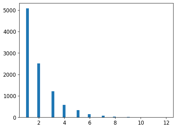
geom_distrib=geom(0.5).rvs(10000, random_state=42)
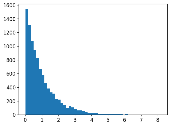
expon_distrib=expon(scale=1).rvs(10000, random_state=42)
plt.hist(geom_distrib, bins=50)
plt.show()
plt.hist(expon_distrib, bins=50)
plt.show()
연습문제 풀이
1.서포트 벡터 머신 회귀(sklearn.svm.SVR)를 kernel=“linear”(하이퍼파라미터 C를 바꿔가며)나 kernel=“rbf”(하이퍼파라미터 C와 gamma를 바꿔가며) 등의 다양한 하이퍼파라미터 설정으로 시도해보세요. 지금은 이 하이퍼파라미터가 무엇을 의미하는지 너무 신경 쓰지 마세요. 최상의 SVR 모델은 무엇인가요?
경고: 사용하는 하드웨어에 따라 다음 셀을 실행하는데 30분 또는 그 이상 걸릴 수 있습니다.
from sklearn.svm import SVR
from sklearn.model_selection import GridSearchCV

param_grid=[
    {'kernel': ['linear'], 'C': [10., 30., 100., 300., 1000., 3000., 10000., 30000.0]},
        {'kernel': ['rbf'], 'C': [1.0, 3.0, 10., 30., 100., 300., 1000.0], 'gamma': [0.01, 0.03, 0.1, 0.3, 1.0, 3.0]},
]

svr_reg = SVR()
grid_search=GridSearchCV(svr_reg, param_grid=param_grid, cv=5,  scoring='neg_mean_squared_error', verbose=2)
grid_search.fit(housing_prepared, housing_labels) # 탐색 과정 출력 생략
Fitting 5 folds for each of 50 candidates, totalling 250 fits
[CV] END ..............................C=10.0, kernel=linear; total time=   6.7s
[CV] END ..............................C=10.0, kernel=linear; total time=   6.7s
[CV] END ..............................C=10.0, kernel=linear; total time=   6.7s
  .
  .
  .

GridSearchCV(cv=5, estimator=SVR(),
             param_grid=[{'C': [10.0, 30.0, 100.0, 300.0, 1000.0, 3000.0,
                                10000.0, 30000.0],
                          'kernel': ['linear']},
                         {'C': [1.0, 3.0, 10.0, 30.0, 100.0, 300.0, 1000.0],
                          'gamma': [0.01, 0.03, 0.1, 0.3, 1.0, 3.0],
                          'kernel': ['rbf']}],
             scoring='neg_mean_squared_error', verbose=2)
최상 모델의 (5-폴드 교차 검증으로 평가한) 점수는 다음과 같다:
negative_mse = grid_search_search.best_score_
rmse = np.sqrt(-negative_mse)
rmse
70286.61838178603
RandomForestRegressor보다 훨씬 좋지 않음 => 최상의 하이퍼파라미터를 확인:
grid_search.best_params_
{'C': 30000.0, 'kernel': 'linear'}
- 선형 커널이 RBF 커널보다 성능이 나은 것 같다.
C는 테스트한 것 중에 최대값이 선택됨 => 따라서 (작은 값들은 지우고) 더 큰 값의C로 그리드서치를 다시 실행해 보아야 한다.(아마도 더 큰 값의C에서 성능이 높아질 것이다)
2.GridSearchCV를 RandomizedSearchCV로 바꿔보세요.
경고: 사용하는 하드웨어에 따라 다음 셀을 실행하는데 45분 또는 그 이상 걸릴 수 있습니다.
from sklearn.model_selection import RandomizedSearchCV
from scipy.stats import expon, reciprocal

# expon(), reciprocal()와 그외 다른 확률 분포 함수에 대해서는
# https://docs.scipy.org/doc/scipy/reference/stats.html를 참고하세요.

# 노트: kernel 매개변수가 "linear"일 때는 gamma가 무시됩니다.
param_distribs = {
        'kernel': ['linear', 'rbf'],
        'C': reciprocal(20, 200000),
        'gamma': expon(scale=1.0),
    }

svm_reg = SVR()
rnd_search = RandomizedSearchCV(svm_reg, param_distributions=param_distribs,
                                n_iter=50, cv=5, scoring='neg_mean_squared_error',
                                verbose=2, random_state=42)
rnd_search.fit(housing_prepared, housing_labels)# 탐색 과정 출력 생략
Fitting 5 folds for each of 50 candidates, totalling 250 fits
[CV] END C=629.782329591372, gamma=3.010121430917521, kernel=linear; total time=   6.9s
[CV] END C=629.782329591372, gamma=3.010121430917521, kernel=linear; total time=   6.7s
[CV] END C=629.782329591372, gamma=3.010121430917521, kernel=linear; total time=   6.9s
  .
  .
  .
RandomizedSearchCV(cv=5, estimator=SVR(), n_iter=50,
                   param_distributions={'C': <scipy.stats._distn_infrastructure.rv_frozen object at 0x00000242513FEFC8>,
                                        'gamma': <scipy.stats._distn_infrastructure.rv_frozen object at 0x000002421647B088>,
                                        'kernel': ['linear', 'rbf']},
                   random_state=42, scoring='neg_mean_squared_error',
                   verbose=2)
최상 모델의 (5-폴드 교차 검증으로 평가한) 점수는 다음과 같다:
negative_mse=rnd_search.best_score_
rmse=np.sqrt(-negative_mse)
rmse
54751.69009256622
이제 RandomForestRegressor의 성능에 훨씬 가까워졌다(하지만 아직 차이가 남). 최상의 하이퍼파라미터를 확인:
rnd_search.best_params_
{'C': 157055.10989448498, 'gamma': 0.26497040005002437, 'kernel': 'rbf'}
이번에는 RBF 커널에 대해 최적의 하이퍼파라미터 조합을 찾았다. 보통 랜덤서치가 같은 시간안에 그리드서치보다 더 좋은 하이퍼파라미터를 찾는다.
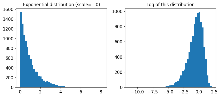
여기서 사용된 scale=1.0인 지수 분포를 살펴보겠다. 일부 샘플은 1.0보다 아주 크거나 작다. 하지만 로그 분포를 보면 대부분의 값이 exp(-2)와 exp(+2), 즉 0.1과 7.4 사이에 집중되어 있음을 알 수 있다.
expon_distrib = expon(scale=1.)
samples = expon_distrib.rvs(10000, random_state=42)
plt.figure(figsize=(10, 4))
plt.subplot(121)
plt.title("Exponential distribution (scale=1.0)")
plt.hist(samples, bins=50)
plt.subplot(122)
plt.title("Log of this distribution")
plt.hist(np.log(samples), bins=50)
plt.show()
C에 사용된 분포는 매우 다르다. 주어진 범위안에서 균등 분포로 샘플링된다. 그래서 오른쪽 로그 분포가 거의 일정하게 나타난다. 이런 분포는 원하는 스케일이 정확이 무엇인지 모를 때 사용하면 좋다:
reciprocal_distrib = reciprocal(20, 200000)
samples = reciprocal_distrib.rvs(10000, random_state=42)
plt.figure(figsize=(10, 4))
plt.subplot(121)
plt.title("Reciprocal distribution (scale=1.0)")
plt.hist(samples, bins=50)
plt.subplot(122)
plt.title("Log of this distribution")
plt.hist(np.log(samples), bins=50)
plt.show()
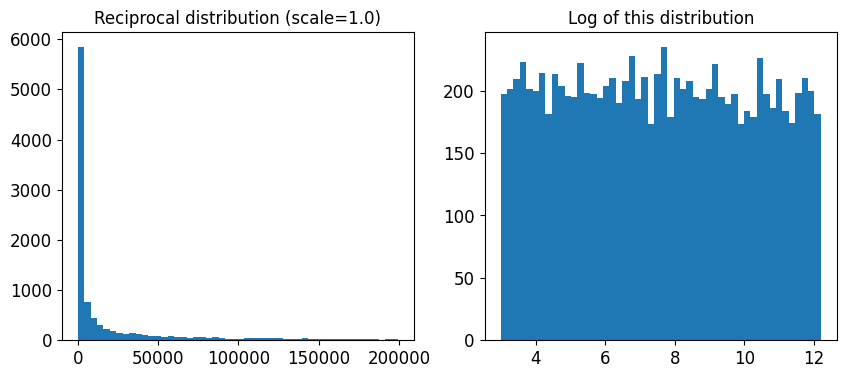
reciprocal() 함수는 하이퍼파라미터의 스케일에 대해 전혀 감을 잡을 수 없을 때 사용한다(오른쪽 그래프에서 볼 수 있듯이 주어진 범위안에서 모든 값이 균등하다). 반면 지수 분포는 하이퍼파라미터의 스케일을 (어느정도) 알고 있을 때 사용하는 것이 좋다.
3.가장 중요한 특성을 선택하는 변환기를 준비 파이프라인에 추가해보세요.
from sklearn.base import BaseEstimator, TransformerMixin

def indices_of_top_k(arr, k):
    return np.sort(np.argpartition(np.array(arr), -k)[-k:])

class TopFeatureSelector(BaseEstimator, TransformerMixin):
    def __init__(self, feature_importances, k):
        self.feature_importances = feature_importances
        self.k = k
    def fit(self, X, y=None):
        self.feature_indices_ = indices_of_top_k(self.feature_importances, self.k)
        return self
    def transform(self, X):
        return X[:, self.feature_indices_]
노트: 이 특성 선택 클래스는 이미 어떤 식으로든 특성 중요도를 계산했다고 가정합니다(가령 RandomForestRegressor을 사용하여). TopFeatureSelector의 fit() 메서드에서 직접 계산할 수도 있지만 (캐싱을 사용하지 않을 경우) 그리드서치나 랜덤서치의 모든 하이퍼파라미터 조합에 대해 계산이 일어나기 때문에 매우 느려집니다.
선택할 특성의 개수를 지정:
k = 5
최상의 k개 특성의 인덱스를 확인:
top_k_feature_indices = indices_of_top_k(feature_importances, k)
top_k_feature_indices
array([ 0, 1, 7, 9, 12], dtype=int64)
np.array(attributes)[top_k_feature_indices]
array(['longitude', 'latitude', 'median_income', 'pop_per_hhold',
       'INLAND'], dtype='<U18')
최상의 k개 특성이 맞는지 다시 확인:
sorted(zip(feature_importances, attributes), reverse=True)[:k]
[(0.3790092248170967, 'median_income'),
 (0.16570630316895876, 'INLAND'),
 (0.10703132208204355, 'pop_per_hhold'),
 (0.06965425227942929, 'longitude'),
 (0.0604213840080722, 'latitude')]
이제 이전에 정의한 준비 파이프라인과 특성 선택기를 추가한 새로운 파이프라인을 만듦:
preparation_and_feature_selection_pipeline = Pipeline([
    ('preparation', full_pipeline),
    ('feature_selection', TopFeatureSelector(feature_importances, k))
])
housing_prepared_top_k_features = preparation_and_feature_selection_pipeline.fit_transform(housing)
처음 3개 샘플의 특성을 확인:
housing_prepared_top_k_features[0:3]
array([[-0.94135046,  1.34743822, -0.8936472 ,  0.00622264,  1.        ],
       [ 1.17178212, -1.19243966,  1.292168  , -0.04081077,  0.        ],
       [ 0.26758118, -0.1259716 , -0.52543365, -0.07537122,  1.        ]])
최상의 k개 특성이 맞는지 다시 확인:
housing_prepared[0:3, top_k_feature_indices]
array([[-0.94135046,  1.34743822, -0.8936472 ,  0.00622264,  1.        ],
       [ 1.17178212, -1.19243966,  1.292168  , -0.04081077,  0.        ],
       [ 0.26758118, -0.1259716 , -0.52543365, -0.07537122,  1.        ]])
4.전체 데이터 준비 과정과 최종 예측을 하나의 파이프라인으로 만들어보세요.
rnd_search.best_params_={'C': 157055.10989448498, 'gamma': 0.26497040005002437, 'kernel': 'rbf'}
rnd_search.best_params_
{'C': 157055.10989448498, 'gamma': 0.26497040005002437, 'kernel': 'rbf'}
prepare_select_and_predict_pipeline = Pipeline([
    ('preparation', full_pipeline),
    ('feature_selection', TopFeatureSelector(feature_importances, k)),
    ('svm_reg', SVR(**rnd_search.best_params_))
])
prepare_select_and_predict_pipeline.fit(housing, housing_labels)
Pipeline(steps=[('preparation',
                 ColumnTransformer(transformers=[('num',
                                                  Pipeline(steps=[('imputer',
                                                                   SimpleImputer(strategy='median')),
                                                                  ('attribs_adder',
                                                                   CombinedAttributesAdder()),
                                                                  ('std_scaler',
                                                                   StandardScaler())]),
                                                  ['longitude', 'latitude',
                                                   'housing_median_age',
                                                   'total_rooms',
                                                   'total_bedrooms',
                                                   'population', 'households',
                                                   'median_income']),
                                                 ('cat', OneHotEncoder(...
                 TopFeatureSelector(feature_importances=array([6.96542523e-02, 6.04213840e-02, 4.21882202e-02, 1.52450557e-02,
       1.55545295e-02, 1.58491147e-02, 1.49346552e-02, 3.79009225e-01,
       5.47789150e-02, 1.07031322e-01, 4.82031213e-02, 6.79266007e-03,
       1.65706303e-01, 7.83480660e-05, 1.52473276e-03, 3.02816106e-03]),
                                    k=5)),
                ('svm_reg',
                 SVR(C=157055.10989448498, gamma=0.26497040005002437))])
몇 개의 샘플에 전체 파이프라인을 적용:
some_data=housing.iloc[0:4]
some_labels=housing_labels.iloc[0:4]

print("Predictions:\t", prepare_select_and_predict_pipeline.predict(some_data))
print("Labels:\t\t", list(some_labels))
Predictions:	 [ 83384.49158095 299407.90439234  92272.03345144 150173.16199041]
Labels:		 [72100.0, 279600.0, 82700.0, 112500.0]
전체 파이프라인이 잘 작동하는 것 같다. 물론 예측 성능이 아주 좋지는 않는다. SVR보다 RandomForestRegressor가 더 나은 것 같다.
5.GridSearchCV를 사용해 준비 단계의 옵션을 자동으로 탐색해보세요.
경고: 사용하는 하드웨어에 따라 다음 셀을 실행하는데 45분 또는 그 이상 걸릴 수 있습니다.
노트: 아래 코드에서 훈련 도중 경고를 피하기 위해 OneHotEncoder의 handle_unknown 하이퍼파라미터를 'ignore'로 지정했습니다. 그렇지 않으면 OneHotEncoder는 기본적으로 handle_unkown='error'를 사용하기 때문에 데이터를 변활할 때 훈련할 때 없던 범주가 있으면 에러를 냅니다. 기본값을 사용하면 훈련 세트에 모든 카테고리가 들어 있지 않은 폴드를 평가할 때 GridSearchCV가 에러를 일으킵니다. 'ISLAND' 범주에는 샘플이 하나이기 때문에 일어날 가능성이 높습니다. 일부 폴드에서는 테스트 세트 안에 포함될 수 있습니다. 따라서 이런 폴드는 GridSearchCV에서 무시하여 피하는 것이 좋습니다.
full_pipeline.named_transformers_["cat"].handle_unknown = 'ignore'

param_grid = [{
    'preparation__num__imputer__strategy': ['mean', 'median', 'most_frequent'],
    'feature_selection__k': list(range(1, len(feature_importances) + 1))
}]

grid_search_prep = GridSearchCV(prepare_select_and_predict_pipeline, param_grid, cv=5,
                                scoring='neg_mean_squared_error', verbose=2)
grid_search_prep.fit(housing, housing_labels) # 경고 메시지, 탐색 과정 삭제
Fitting 5 folds for each of 48 candidates, totalling 240 fits
  .
  .
  .
GridSearchCV(cv=5,
             estimator=Pipeline(steps=[('preparation',
                                        ColumnTransformer(transformers=[('num',
                                                                         Pipeline(steps=[('imputer',
                                                                                          SimpleImputer(strategy='median')),
                                                                                         ('attribs_adder',
                                                                                          CombinedAttributesAdder()),
                                                                                         ('std_scaler',
                                                                                          StandardScaler())]),
                                                                         ['longitude',
                                                                          'latitude',
                                                                          'housing_median_age',
                                                                          'total_rooms',
                                                                          'total_bedrooms',
                                                                          'population',
                                                                          'households',
                                                                          'median_inc...
       5.47789150e-02, 1.07031322e-01, 4.82031213e-02, 6.79266007e-03,
       1.65706303e-01, 7.83480660e-05, 1.52473276e-03, 3.02816106e-03]),
                                                           k=5)),
                                       ('svm_reg',
                                        SVR(C=157055.10989448498,
                                            gamma=0.26497040005002437))]),
             param_grid=[{'feature_selection__k': [1, 2, 3, 4, 5, 6, 7, 8, 9,
                                                   10, 11, 12, 13, 14, 15, 16],
                          'preparation__num__imputer__strategy': ['mean',
                                                                  'median',
                                                                  'most_frequent']}],
             scoring='neg_mean_squared_error', verbose=2)
grid_search_prep.best_params_
{'feature_selection__k': 1, 'preparation__num__imputer__strategy': 'mean'}
최상의 Imputer 정책은 most_frequent이고 거의 모든 특성이 유용(16개 중 15개). 마지막 특성(ISLAND)은 잡음이 추가될 뿐이다.
출처
- 핸즈온 머신러닝 2판