3. 분류
in ML/DL / Handson-ml2
핸즈온 머신러닝 2판에서 공부했던 내용을 정리하는 부분입니다.
MNIST 데이터셋을 통해 분류시스템 집중적으로 분석
설정
# 파이썬 ≥3.5 필수
import sys
assert sys.version_info >= (3, 5)

# 사이킷런 ≥0.20 필수
import sklearn
assert sklearn.__version__ >= "0.20"

# 공통 모듈 임포트
import numpy as np
import os

# 노트북 실행 결과를 동일하게 유지하기 위해
np.random.seed(42)

# 깔끔한 그래프 출력을 위해
%matplotlib inline
import matplotlib as mpl
import matplotlib.pyplot as plt
mpl.rc('axes', labelsize=14)
mpl.rc('xtick', labelsize=12)
mpl.rc('ytick', labelsize=12)

# 그림을 저장할 위치
PROJECT_ROOT_DIR = "."
CHAPTER_ID = "classification"
IMAGES_PATH = os.path.join(PROJECT_ROOT_DIR, "images", CHAPTER_ID)
os.makedirs(IMAGES_PATH, exist_ok=True)

def save_fig(fig_id, tight_layout=True, fig_extension="png", resolution=300):
    path = os.path.join(IMAGES_PATH, fig_id + "." + fig_extension)
    print("그림 저장:", fig_id)
    if tight_layout:
        plt.tight_layout()
    plt.savefig(path, format=fig_extension, dpi=resolution)
3.1 MNIST
- 고등학생과 미국 조사국 직원들이 손으로 쓴 70,000개의 작은 숫자 이미지 데이터셋
- 머신러닝 분야의 ‘Hello World’, 분류 학습용으로 많이 쓰임
from sklearn.datasets import fetch_openml
mnist=fetch_openml('mnist_784', version=1, as_frame=False)
mnist.keys()
dict_keys(['data', 'target', 'frame', 'categories', 'feature_names', 'target_names', 'DESCR', 'details', 'url'])
- 사이킷런에서 읽어들인 데이터셋의 특징
- DESCR 키: 데이터셋을 설명
- data 키: 샘플이 행, 특성이 열로 이루어진 배열
- target 키: 레이블 배열
X, y = mnist["data"], mnist["target"]
X.shape
(70000, 784)
y.shape
(70000,)
28*28
784
- 이미지: 70,000개 / 특성: 784개 / 이미지 28 X 28 픽셀
%matplotlib inline
import matplotlib as mpl
import matplotlib.pyplot as plt

some_digit = X[0]
some_digit_image = some_digit.reshape(28,28)
plt.imshow(some_digit_image, cmap=mpl.cm.binary)

save_fig("some_digit_plot")
plt.show()
그림 저장: some_digit_plot
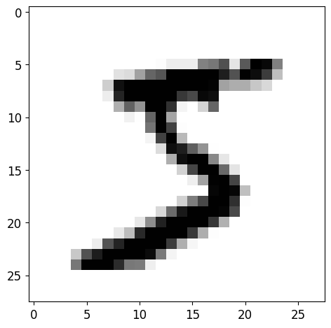
y[0]
'5'
y=y.astype(np.uint8)
def plot_digit(data):
    image = data.reshape(28,28)
    plt.imshow(image, cmap=mpl.cm.binary, interpolation="nearest")
    plt.axis("off")
# 숫자 그림을 위한 추가 함수
def plot_digits(instances, images_per_row=10, **options):
    size=28
    images_per_row= min(len(instances), images_per_row)
    n_rows=(len(instances)-1) // images_per_row + 1

    # 필요하면 그리드 끝을 채우기 위해 빈 이미지를 추가합니다:
    n_empty=n_rows*images_per_row - len(instances)
    padded_instances= np.concatenate([instances, np.zeros((n_empty, size*size))], axis=0)

    # 배열의 크기를 바꾸어 28×28 이미지를 담은 그리드로 구성합니다:
    image_grid = padded_instances.reshape((n_rows, images_per_row, size, size))

    # 축 0(이미지 그리드의 수직축)과 2(이미지의 수직축)를 합치고 축 1과 3(두 수평축)을 합칩니다.
    # 먼저 transpose()를 사용해 결합하려는 축을 옆으로 이동한 다음 합칩니다:
    big_image = image_grid.transpose(0, 2, 1, 3).reshape(n_rows * size,
                                                         images_per_row * size)
    # 하나의 큰 이미지를 얻었으므로 출력하면 됩니다:
    plt.imshow(big_image, cmap = mpl.cm.binary, **options)
    plt.axis("off")
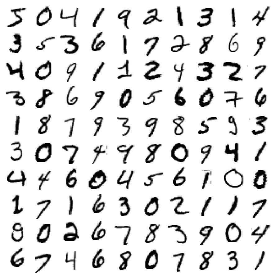
plt.figure(figsize=(9,9))
example_images=X[:100]
plot_digits(example_images, images_per_row=10)
save_fig("more_digits_plot")
plt.show()
그림 저장: more_digits_plot
y[0]
5
X_train, y_train, X_test, y_test = X[:60000], y[:60000], X[60000:], y[60000:]
- 훈련 세트: 앞쪽 60,000개 / 테스트 세트: 뒤쪽 10,000개 → 훈련 세트 이미 섞여서 모든 교차 검증 폴드 비슷하게 만듦
- 어떤 학습 알고리즘은 훈련 샘플 순서에 민감 → 데이터셋을 섞으면 이런 문제 방지 가능
3.2 이진 분류기 훈련
y_train_5=(y_train==5)
y_test_5=(y_test==5)
- 이진 분류기 → ex) 5와 5아님 두개의 클래스로 분류
from sklearn.linear_model import SGDClassifier

sgd_clf=SGDClassifier(random_state=42)
sgd_clf.fit(X_train, y_train_5)
SGDClassifier(random_state=42)
sgd_clf.predict([some_digit])
array([ True])
from sklearn.model_selection import cross_val_score

cross_val_score(sgd_clf, X_train, y_train_5, cv=3, scoring="accuracy")
array([0.95035, 0.96035, 0.9604 ])
- SGD 분류기(Stochastic Gradient Descent Classifier)
- 매우 큰 데이터 셋을 효율적으로 처리 → 한번에 하나씩 훈련 샘플을 독립적으로 처리하기 때문(온라인 학습에 적합)
TIP
SGD classifier는 훈련에 무작위성 사용 → 결과 재현을 위해서는 random_state 매개변수 지정
- 매우 큰 데이터 셋을 효율적으로 처리 → 한번에 하나씩 훈련 샘플을 독립적으로 처리하기 때문(온라인 학습에 적합)
3.3 성능 측정
3.3.1 교차 검증을 사용한 정확도 측정
from sklearn.model_selection import StratifiedKFold
from sklearn.base import clone

# shuffle=False가 기본값이기 때문에 random_state를 삭제하던지 shuffle=True로 지정하라는 경고가 발생합니다.
# 0.24버전부터는 에러가 발생할 예정이므로 향후 버전을 위해 shuffle=True을 지정합니다.

skfolds=StratifiedKFold(n_splits=3, random_state=42, shuffle=True)

for train_index, test_index in skfolds.split(X_train, y_train_5):
    clone_clf=clone(sgd_clf)
    X_train_folds=X_train[train_index]
    y_train_folds=y_train_5[train_index]
    X_test_fold=X_train[test_index]
    y_test_fold = y_train_5[test_index]

    clone_clf.fit(X_train_folds, y_train_folds)
    y_pred=clone_clf.predict(X_test_fold)
    n_correct=sum(y_pred == y_test_fold)
    print(n_correct / len(y_pred))
0.9669
0.91625
0.96785
- StratifiedKFold: 클래스별 비율이 유지되도록 폴드를 만들기 위해 계층적 샘플링 수행
from sklearn.model_selection import cross_val_score
cross_val_score(sgd_clf, X_train, y_train_5, cv=3, scoring="accuracy")
array([0.95035, 0.96035, 0.9604 ])
- cross_val_score() 3개의 폴드 교차 검증으로 SGD classifier 평가 → 모든 교차 검증 폴드에 대해 95%이상의 정확도
from sklearn.base import BaseEstimator

class Never5Classifier(BaseEstimator):
    def fit(self, X, y=None):
        pass
    def predict(self, X):
        return np.zeros((len(X), 1), dtype=bool)
never_5_clf=Never5Classifier()
cross_val_score(never_5_clf, X_train, y_train_5, cv=3, scoring='accuracy')
array([0.91125, 0.90855, 0.90915])
- 정확도 90%이상으로 나옴 → 이미지의 10% 정도만 숫자 5이기 때문에 무조건 ‘5 아님’으로 예측하면 정확도 90%
이 예제는 정확도를 분류기의 성능 측정 지표로 사용하지 않는 이유 보여줌 → 특히 불균형한 데이터셋 사용 시 더욱 그렇다.
- 노트: 이 출력(그리고 이 노트북과 다른 노트북의 출력)이 책의 내용과 조금 다를 수 있다.
- 첫째, 사이킷런과 다른 라이브러리들이 발전하면서 알고리즘이 조금씩 변경되기 때문에 얻어지는 결괏값이 바뀔 수 있다. 최신 사이킷런 버전을 사용한다면(일반적으로 권장됨) 책이나 이 노트북을 만들 때 사용한 버전과 다를 것이므로 차이가 남
- 둘째, 많은 훈련 알고리즘은 확률적이다. 즉 무작위성에 의존한다. 이론적으로 의사 난수를 생성하도록 난수 생성기에 시드 값을 지정하여 일관된 결과를 얻을 수 있다(random_state=42나 np.random.seed(42)를 종종 보게 되는 이유). 하지만 여기에서 언급한 다른 요인으로 인해 충분하지 않을 때가 있다.
- 셋째, 훈련 알고리즘이 여러 스레드(C로 구현된 알고리즘)나 여러 프로세스(예를 들어 n_jobs 매개변수를 사용할 때)로 실행되면 연산이 실행되는 정확한 순서가 항상 보장되지 않는다. 따라서 결괏값이 조금 다를 수 있다.
- 마지막으로, 여러 세션에 결쳐 순서가 보장되지 않는 파이썬 딕셔너리(dict)이나 셋(set) 같은 것은 완벽한 재현성이 불가능하다. 또한 디렉토리 안에 있는 파일의 순서도 보장되지 않는다.
3.3.2 오차 행렬
- 분류기 성능 평가로 더 좋은 방법: 클래스 A의 샘플이 클래스 B로 분류된 횟수 측정
- ex) 숫자 5의 이미지를 3으로 잘못 분류한 횟수 → 오차 행렬 5행 3열
from sklearn.model_selection import cross_val_predict

y_train_pred= cross_val_predict(sgd_clf, X_train, y_train_5, cv=3)
from sklearn.metrics import confusion_matrix

confusion_matrix(y_train_5, y_train_pred)
array([[53892,   687],
       [ 1891,  3530]], dtype=int64)
- 오차 행렬 만들려면 예측 값이 있어야함 → cross_val_predict() 함수 사용
- 교차검증 수행하여 각 테스트 폴드에서 얻은 예측 반환
- 즉, 훈련 샘플에 대해 깨끗한 예측을 얻게 됨 (모델이 훈련동안 보지 못한 샘플에 대해서 예측했다는 뜻)
- 오차 행렬의 구성
행: 실제 클래스 / 열: 예측 클래스
TN(진짜 음성) FP(거짓양성) FN(거짓 음성) TP(진짜 양성) 정밀도(Precision): 양성 예측의 정확도 \[\begin{align*} & 정밀도 = \frac{TP}{TP+FP} \end{align*}\]
재현율(Recall): 분류기가 정확하게 감지한 양성 샘플의 비율 → 민감도(sensitivity), 진짜양성 비율(TPR) \[\begin{align*} & 재현율 = \frac{TP}{TP+FN} \end{align*}\]
y_train_perfect_predictions = y_train_5 # 완벽한 분류기일 경우
confusion_matrix(y_train_5, y_train_perfect_predictions)
array([[54579,     0],
       [    0,  5421]], dtype=int64)
3.3.3 정밀도와 재현율
from sklearn.metrics import precision_score, recall_score

precision_score(y_train_5, y_train_pred)
0.8370879772350012
cm=confusion_matrix(y_train_5, y_train_pred)
cm[1,1] / (cm[0,1]+cm[1,1])
0.8370879772350012
recall_score(y_train_5, y_train_pred)
0.6511713705958311
cm[1,1] / (cm[1,0]+cm[1,1])
0.6511713705958311
- precision: 0.837, recall: 0.651 → 5로 판별된 이미지 중에서 83.7%만 정확, 전체 숫자 5에서 65.1%만 감지
from sklearn.metrics import f1_score

f1_score(y_train_5, y_train_pred)
0.7325171197343846
cm[1, 1] / (cm[1, 1] + (cm[1, 0] + cm[0, 1]) / 2)
0.7325171197343847
- F1 score
- 두 분류기 비교할 때 좋음
- 정밀도, 재현율 비슷하면 F1 score 높다 → 항상 바람직한 것은 아님
- 정밀도 재현율 트레이드오프: 정밀도를 올리면 재현율이 낮아지고 그 반대도 일어나는 것
3.3.4 정밀도/재현율 트레이드오프
- SGDClassifier 분류 진행 방법과 트레이드오프 이해
y_scores=sgd_clf.decision_function([some_digit])
y_scores
array([2164.22030239])
threshold=0
y_some_digit_pred=(y_scores>threshold)
y_some_digit_pred
array([ True])
threshold=8000
y_some_digit_pred=(y_scores>threshold)
y_some_digit_pred
array([False])
- 결정 함수(decision function)을 사용하여 각 샘플의 점수 계산 → 사이킷런의 decision_function()함수로 예측에 사용한 점수 확인 가능
- 결정 임곗값(decision threshold): 이 값보다 점수가 크면 양성 클래스, 작으면 음성 클래스
y_scores=cross_val_predict(sgd_clf, X_train, y_train_5, cv=3, method='decision_function')
- cross_val_predict() 함수로 모든 샘플의 점수 구함
from sklearn.metrics import precision_recall_curve

precisions, recalls, thresholds =precision_recall_curve(y_train_5, y_scores)
- precision_recall_curve() 함수를 사용하여 가능한 모든 임곗값에 대해 정밀도와 재현율 계산 가능
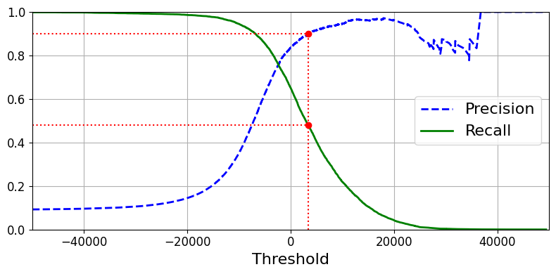
def plot_precision_recall_vs_threshold(precisions, recalls, thresholds):
    plt.plot(thresholds, precisions[:-1], "b--", label="Precision", linewidth=2)
    plt.plot(thresholds, recalls[:-1], "g-", label="Recall", linewidth=2)
    plt.legend(loc="center right", fontsize=16) # Not shown in the book
    plt.xlabel("Threshold", fontsize=16)        # Not shown
    plt.grid(True)                              # Not shown
    plt.axis([-50000, 50000, 0, 1])             # Not shown


recall_90_precision = recalls[np.argmax(precisions >= 0.90)]
threshold_90_precision = thresholds[np.argmax(precisions >= 0.90)]


plt.figure(figsize=(8, 4))                                                                  # Not shown
plot_precision_recall_vs_threshold(precisions, recalls, thresholds)
plt.plot([threshold_90_precision, threshold_90_precision], [0., 0.9], "r:")                 # Not shown
plt.plot([-50000, threshold_90_precision], [0.9, 0.9], "r:")                                # Not shown
plt.plot([-50000, threshold_90_precision], [recall_90_precision, recall_90_precision], "r:")# Not shown
plt.plot([threshold_90_precision], [0.9], "ro")                                             # Not shown
plt.plot([threshold_90_precision], [recall_90_precision], "ro")                             # Not shown
save_fig("precision_recall_vs_threshold_plot")                                              # Not shown
plt.show()
그림 저장: precision_recall_vs_threshold_plot
(y_train_pred==(y_scores>0)).all()
True
NOTE
- 정밀도 곡선이 재현율 곡선보다 울퉁불퉁한 이유 → 임계값을 올리더라도 정밀도가 가끔 낮아질 때가 있다
def plot_precision_vs_recall(precisios, recalls):
    plt.plot(recalls, precisions, 'b-', linewidth=2)
    plt.xlabel('Recall', fontsize=16)
    plt.ylabel('Precision', fontsize=16)
    plt.axis([0,1,0,1])
    plt.grid(True)

plt.figure(figsize=(8,6))
plot_precision_vs_recall(precisions, recalls)
plt.plot([recall_90_precision, recall_90_precision], [0.,0.9], 'r:')
plt.plot([0.0,recall_90_precision],[0.9,0.9],'r:')
plt.plot([recall_90_precision], [0.9], 'ro')
save_fig("precision_vs_recall_plot")
plt.show()
그림 저장: precision_vs_recall_plot
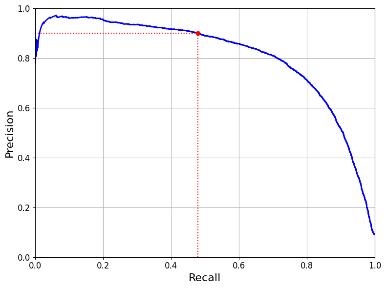
- 재현율에 대한 정밀도 곡선 그리기
- average_precision_score() 함수를 사용하면 정밀도/재현율 곡선 아래 면적을 구할 수 있어서 서로 다른 두 모델 비교에 좋음
- 재현율 80%근처에서 정밀도 급격히 감소 → 이 하강점 직전을 트레이드오프로 선택하는 것이 좋음
threshold_90_precision=thresholds[np.argmax(precisions>=0.90)]
threshold_90_precision
3370.0194991439594
y_train_pred_90=(y_scores>=threshold_90_precision)
precision_score(y_train_5, y_train_pred_90)
0.9000345901072293
recall_score(y_train_5, y_train_pred_90)
0.4799852425751706
- 정밀도 90% 분류기 생성 → 최소한 90%의 정밀도가 되는 가장 낮은 임계점 찾음
- 충분히 큰 임계값을 지정하면 끝 → 재현율이 너무 낮다면 유용하지 않다
3.3.5 ROC 곡선
- 수신기 조작 특성(receiver operating characteristic) 곡선
- 이진 분류에 널리 사용됨
- 거짓 양성 비율(FPR)에 대한 진짜 양성 비율(TPR, 재현율의 다른 이름)
- FPR=1-TNR → ROC 곡선= 민감도(재현율)에 대한 1-특이도 그래프
- TNR(진짜 음성 비율, 특이도)
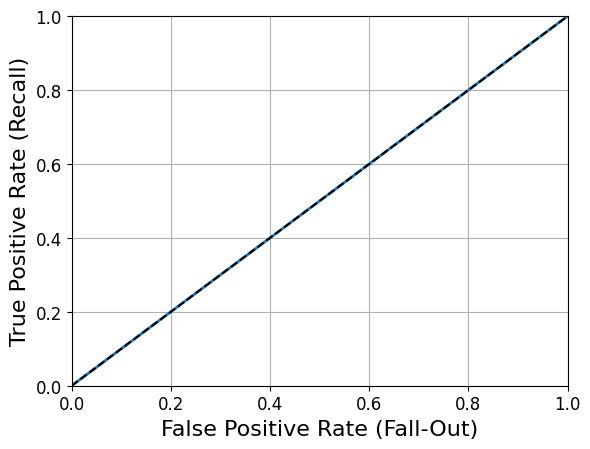
from sklearn.metrics import roc_curve

fpr, tpr, thresholds = roc_curve(y_train_5, y_scores)
def plot_roc_curve(fpr, tpr, label=None):
    plt.plot(fpr, tpr, linewidth=2, label=label)
    plt.plot([0, 1], [0, 1], 'k--') # 대각 점선
    plt.axis([0, 1, 0, 1])                                    # Not shown in the book
    plt.xlabel('False Positive Rate (Fall-Out)', fontsize=16) # Not shown
    plt.ylabel('True Positive Rate (Recall)', fontsize=16)    # Not shown
    plt.grid(True)                                            # Not shown

plt.figure(figsize=(8, 6))                                    # Not shown
plot_roc_curve(fpr, tpr)
fpr_90 = fpr[np.argmax(tpr >= recall_90_precision)]           # Not shown
plt.plot([fpr_90, fpr_90], [0., recall_90_precision], "r:")   # Not shown
plt.plot([0.0, fpr_90], [recall_90_precision, recall_90_precision], "r:")  # Not shown
plt.plot([fpr_90], [recall_90_precision], "ro")               # Not shown
save_fig("roc_curve_plot")                                    # Not shown
plt.show()
그림 저장: roc_curve_plot
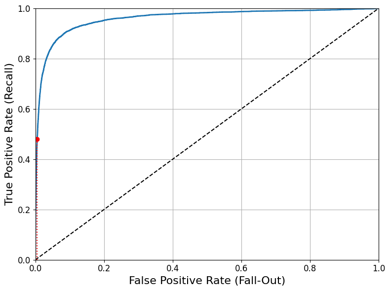
- 트레이드오프 존재: TPR(재현율)이 높을수록 분류기가 만드는 거짓 양성(FPR)이 늘어남
점선=완전한 랜덤 분류기의 ROC 곡선 → 좋은 분류기는 이 점선에서 최대한 멀리 떨어져야함(왼쪽 위 모서리)
- 곡선 아래의 면적(AUC)을 측정하여 분류기들 비교 가능 → 완벽한 분류기:1, 완전한 랜덤 분류기: 0.5
from sklearn.metrics import roc_auc_score

roc_auc_score(y_train_5, y_scores)
0.9604938554008616
TIP
- 양성 클래스가 드물거나 거짓 음성보다 거짓 양성이 더 중요할 때 PR곡선(정밀도/재현율) 사용하고 반대의 경우는 ROC곡선 사용
- RandomForestClassifier와 SGDClassifier의 성능 비교
- RandomForestClassifier: 작동 방식 차이로 decision_function() 대신 predict_proba() 사용 (사이킷런 분류기 일반적으로 둘중 하나 혹은 둘다 가지고 있음)
- predict_proba(): 샘플이 행, 클래스가 열이고 샘플이 주어진 클래스에 속할 확률을 담은 배열 반환
노트: 사이킷런 0.22 버전에서 바뀔 기본 값을 사용해 n_estimators=100로 지정합니다.
from sklearn.ensemble import RandomForestClassifier

forest_clf=RandomForestClassifier(n_estimators=100, random_state=42)
y_probas_forest=cross_val_predict(forest_clf, X_train, y_train_5, cv=3, method='predict_proba')
y_scores_forest=y_probas_forest[:,1] # 점수 = 양성 클래스의 확률
fpr_forest, tpr_forest, thresholds_forest=roc_curve(y_train_5, y_scores_forest)
recall_for_forest = tpr_forest[np.argmax(fpr_forest >= fpr_90)]

plt.figure(figsize=(8, 6))
plt.plot(fpr, tpr, "b:", linewidth=2, label="SGD")
plot_roc_curve(fpr_forest, tpr_forest, "Random Forest")
plt.plot([fpr_90, fpr_90], [0., recall_90_precision], "r:")
plt.plot([0.0, fpr_90], [recall_90_precision, recall_90_precision], "r:")
plt.plot([fpr_90], [recall_90_precision], "ro")
plt.plot([fpr_90, fpr_90], [0., recall_for_forest], "r:")
plt.plot([fpr_90], [recall_for_forest], "ro")
plt.grid(True)
plt.legend(loc="lower right", fontsize=16)
save_fig("roc_curve_comparison_plot")
plt.show()
그림 저장: roc_curve_comparison_plot
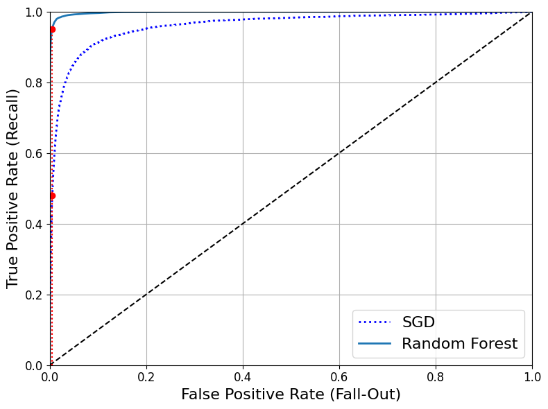
roc_auc_score(y_train_5, y_scores_forest)
0.9983436731328145
y_train_pred_forest=cross_val_predict(forest_clf, X_train, y_train_5, cv=3)
precision_score(y_train_5, y_train_pred_forest)
0.9905083315756169
recall_score(y_train_5, y_train_pred_forest)
0.8662608374838591
- 99.0%의 정밀도, 86.6%의 재현율을 보여줌
3.4 다중 분류
- 다중 분류기: 둘 이상의 클래스 구별 가능
- SGD 분류기, 랜덤 포레스트 분류기, 나이브 베이즈 분류기: 여러개의 클래스 직접 처리 가능
- 로지스틱 회귀, 서포트 벡터 머신: 이진 분류만 가능
- 이진 분류기를 여러개 사용하여 다중 분류 기법
- OvR 전략(OvA 전략): 각 분류기의 결정 점수 중에서 가장 높은 것을 클래스로 선택
- OvO 전략: 각 조합마다 이진 분류기 훈련하여 가장 많이 양성으로 분류된 클래스 선택 → 클래스가 N개이면 분류기 \(\frac{N\times(N-1)}{2}\)개 필요
- 장점: 각 분류기의 훈련에 구별할 수 있는 두 클래스에 해당하는 샘플만 필요
- 서포트 벡터 머신: OvO방식 선호 / 나머지 이진 분류 알고리즘: OvR 방식 선호
- 다중 클래스 분류 작업에 이진 분류 알고리즘 사용 시 → 사이킷런이 자동으로 OvR or OvO 실행
# 서포트 벡터 머신 분류기(자동)
from sklearn.svm import SVC

svm_clf=SVC(gamma='auto', random_state=42)
svm_clf.fit(X_train[:1000], y_train[:1000])
svm_clf.predict([some_digit])
array([5], dtype=uint8)
some_digit_scores=svm_clf.decision_function([some_digit])
some_digit_scores
array([[ 2.81585438,  7.09167958,  3.82972099,  0.79365551,  5.8885703 ,
         9.29718395,  1.79862509,  8.10392157, -0.228207  ,  4.83753243]])
np.argmax(some_digit_scores)
5
svm_clf.classes_
array([0, 1, 2, 3, 4, 5, 6, 7, 8, 9], dtype=uint8)
svm_clf.classes_[5]
5
- 0~9까지의 원래 타깃 클래스를 활용해 SVC 훈련
- 샘플당 클래스 개수만큼의 점수 반환
CAUTION
classes_속성에 타깃 클래스의 리스트를 값으로 정렬하여 저장 → 일반적으로는 위의 예제처럼 인덱스와 클래스 값이 같지 않음
# 서포트 벡터 머신 분류기(OvR 강제)
from sklearn.multiclass import OneVsRestClassifier
ovr_clf=OneVsRestClassifier(SVC(gamma='auto', random_state=42))
ovr_clf.fit(X_train[:1000], y_train[:1000])
ovr_clf.predict([some_digit])
array([5], dtype=uint8)
len(ovr_clf.estimators_)
10
# SGDClassifier
sgd_clf.fit(X_train,y_train)
sgd_clf.predict([some_digit])
array([3], dtype=uint8)
sgd_clf.decision_function([some_digit])
array([[-31893.03095419, -34419.69069632,  -9530.63950739,
          1823.73154031, -22320.14822878,  -1385.80478895,
        -26188.91070951, -16147.51323997,  -4604.35491274,
        -12050.767298  ]])
cross_val_score(sgd_clf, X_train, y_train, cv=3, scoring='accuracy')
array([0.87365, 0.85835, 0.8689 ])
- SGDClassifier: 다중 분류 가능으로 별도의 OvR, OvO 적용 필요 없음
- 모든 테스트 폴드에서 84% 이상얻음
# SGDClassifier(스케일 조정)
from sklearn.preprocessing import StandardScaler
scaler=StandardScaler()
X_train_scaled=scaler.fit_transform(X_train.astype(np.float64))
cross_val_score(sgd_clf, X_train_scaled, y_train, cv=3, scoring='accuracy')
array([0.8983, 0.891 , 0.9018])
3.5 에러 분석
- 가능성 높은 모델 찾았다고 가정 후 모델 성능 향상 방법 찾기 → 에러의 종류 분석
y_train_pred=cross_val_predict(sgd_clf, X_train_scaled, y_train, cv=3)
conf_mx=confusion_matrix(y_train, y_train_pred)
conf_mx
array([[5577,    0,   22,    5,    8,   43,   36,    6,  225,    1],
       [   0, 6400,   37,   24,    4,   44,    4,    7,  212,   10],
       [  27,   27, 5220,   92,   73,   27,   67,   36,  378,   11],
       [  22,   17,  117, 5227,    2,  203,   27,   40,  403,   73],
       [  12,   14,   41,    9, 5182,   12,   34,   27,  347,  164],
       [  27,   15,   30,  168,   53, 4444,   75,   14,  535,   60],
       [  30,   15,   42,    3,   44,   97, 5552,    3,  131,    1],
       [  21,   10,   51,   30,   49,   12,    3, 5684,  195,  210],
       [  17,   63,   48,   86,    3,  126,   25,   10, 5429,   44],
       [  25,   18,   30,   64,  118,   36,    1,  179,  371, 5107]],
      dtype=int64)
사이킷런 0.22 버전부터는 sklearn.metrics.plot_confusion_matrix() 함수를 사용할 수 있습니다.
def plot_confusion_matrix(matrix):
    """If you prefer color and a colorbar"""
    fig = plt.figure(figsize=(8,8))
    ax = fig.add_subplot(111)
    cax = ax.matshow(matrix)
    fig.colorbar(cax)
plt.matshow(conf_mx, cmap=plt.cm.gray)
save_fig("confusion_matrix_plot", tight_layout=False)
plt.show()
그림 저장: confusion_matrix_plot
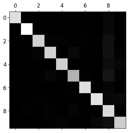
- 숫자 5가 다른 숫자들에 비해 조금 더 어둡다
- 숫자 5의 이미지가 적거나 다른 숫자만큼 잘 분류 못한다는 뜻
row_sums=conf_mx.sum(axis=1, keepdims=True)
norm_conf_mx=conf_mx / row_sums
np.fill_diagonal(norm_conf_mx, 0)
plt.matshow(norm_conf_mx, cmap=plt.cm.gray)
save_fig("confusion_matrix_errors_plot", tight_layout=False)
plt.show()
그림 저장: confusion_matrix_errors_plot
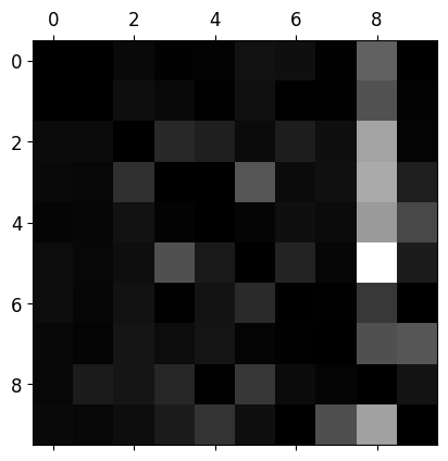
- 행: 실제 클래스, 열: 예측 클래스
- 클래스 8의 열이 상당히 밝음 → 많은 이미지가 8로 잘못 분류됨
- 클래스 8의 행은 나쁘지 않음 → 8은 제대로 분류됨
- 3과 5가 서로 많이 혼동
- 성능 향상 방안에 대한 통찰(8로 잘못 분류되는 것)
- 8처럼 보이는 숫자의 데이터를 더 많이 모아 훈련
- 분류기에 도움이 될만한 특성 찾아봄 → 동심원 수를 세는 알고리즘(8: 2개, 6: 1개, 5: 0개)
- 동심원 같은 어떤 패턴이 드러나도록 이미지 전처리(scikit-Image, Pillow, OpenCV 등 사용)
cl_a, cl_b=3,5
X_aa = X_train[(y_train == cl_a) & (y_train_pred == cl_a)]
X_ab = X_train[(y_train == cl_a) & (y_train_pred == cl_b)]
X_ba = X_train[(y_train == cl_b) & (y_train_pred == cl_a)]
X_bb = X_train[(y_train == cl_b) & (y_train_pred == cl_b)]

plt.figure(figsize=(8,8))
plt.subplot(221); plot_digits(X_aa[:25], images_per_row=5)
plt.subplot(222); plot_digits(X_ab[:25], images_per_row=5)
plt.subplot(223); plot_digits(X_ba[:25], images_per_row=5)
plt.subplot(224); plot_digits(X_bb[:25], images_per_row=5)
save_fig("error_analysis_digits_plot")
plt.show()
그림 저장: error_analysis_digits_plot
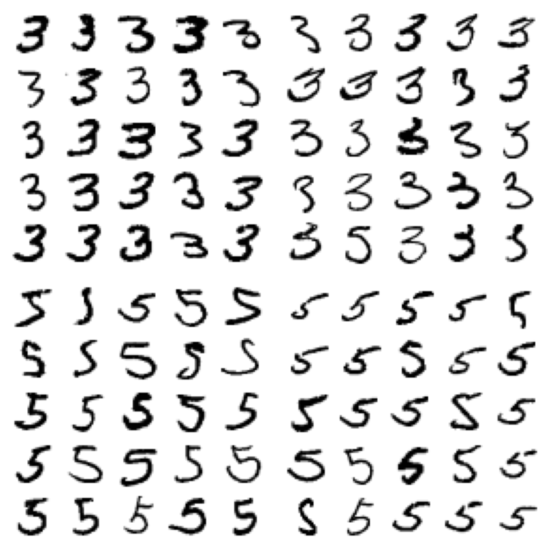
- 왼쪽의 두개: 3으로 분류된 이미지, 오른쪽의 두개: 5로 분류된 두개
- 일부는 잘못 쓰여서 분류가 어렵지만 대부분은 분류기의 실수 및 에러
- SGDClassifier가 단순 선형 모델이기에 쉽게 혼동 → 선형분류기는 클래스마다 픽셀에 가중치를 할당하고 새로운 이미지에 대해 단순히 픽셀 강도의 가중치 합을 클래스의 점수로 계산하기 때문
- 3과 5의 주요 차이인 위아래를 연결하는 작은 직선의 위치를 구별 할 수 있게 이미지 중앙에 위치하고 회전하지 않도록 전처리 필요
3.6 다중 레이블 분류
- ex) 얼굴 인식 분류기 → 앨리스, 밥, 찰리 세 사람의 얼굴 인식: [1,0,1] - 앨리스, 밥이 있는 사진
from sklearn.neighbors import KNeighborsClassifier

y_train_large=(y_train>=7)
y_train_odd=(y_train%2==1)
y_multilabel=np.c_[y_train_large, y_train_odd]

knn_clf=KNeighborsClassifier()
knn_clf.fit(X_train, y_multilabel)
KNeighborsClassifier()
knn_clf.predict([some_digit])
array([[False, True]])
y_train_knn_pred=cross_val_predict(knn_clf, X_train, y_multilabel, cv=3)
f1_score(y_multilabel, y_train_knn_pred, average='macro')
0.976410265560605
- 7이상과 홀수 유무로 분류
- KNeighborsClassifier는 다중 레이블 분류 지원 → 모든 분류기가 그런 것은 아님
- 다중 레이블 분류기 평가 방법 많음(프로젝트에 따라 다름)
- 위의 예제는 모든 레이블 가중치 같다고 가정하고 진행 → 실제는 레이블에 클래스의 지지도를 가중치로 주고 진행(average=’weighted’로 두고 진행)
- 지지도: 타깃 레이블에 속한 샘플 수
- average=’micro’ → 모든 클래스의 FP, FN, TP 총합을 이용해 F1점수 계산
- accuracy_score, precision_score, recall_score, classification_report 함수 등이 다중 분류 지원
3.7 다중 출력 분류
- 다중 레이블 분류에서 한 레이블이 다중 클래스가 될 수 있도록 일반화 한 것(즉, 값을 두개 이상 가질 수 있음)
- 이미지 잡음 제거 시스템
- 입력: 잡음이 많은 숫자 이미지, 출력: MNIST 이미지 처럼 픽셀의 강도를 담은 배열
- 분류기의 출력이 다중 레이블(픽셀당 한 레이블)이고 각 레이블 값은 여러개(0~255) →따라서 다중 출력 분류 시스템
NOTE
- 분류와 회귀의 경계는 모호하다 → 이 예처럼 회귀도 가능하고 샘플마다 클래스와 값을 모두 포함하는 다중 레이블이 출력되는 시스템도 가능
noise=np.random.randint(0, 100, (len(X_train), 784))
X_train_mod=X_train+noise
noise = np.random.randint(0, 100, (len(X_test), 784))
X_test_mod=X_test+noise
y_train_mod=X_train
y_test_mod=X_test
some_index=0
plt.subplot(121); plot_digit(X_test_mod[some_index])
plt.subplot(122); plot_digit(y_test_mod[some_index])
save_fig("noisy_digit_example_plot")
plt.show()
그림 저장: noisy_digit_example_plot
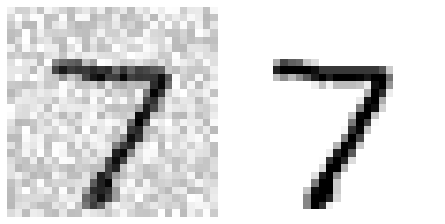
- 테스트 세트에서 이미지 하나 선택(사실 잘못된 것)
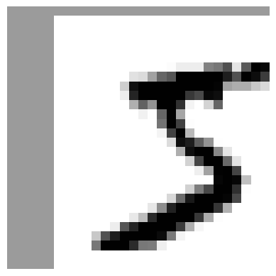
knn_clf.fit(X_train_mod, y_train_mod)
clean_digit=knn_clf.predict([X_test_mod[some_index]])
plot_digit(clean_digit)
save_fig("cleaned_digit_example_plot")
그림 저장: cleaned_digit_example_plot

- 이미지 깨끗하게 만듦 → 타깃과 비슷
추가 내용
더미 (즉 랜덤) 분류기
from sklearn.dummy import DummyClassifier
# 0.24버전부터 strategy의 기본값이 'stratified'에서 'prior'로 바뀌므로 명시적으로 지정합니다.
dmy_clf=DummyClassifier(strategy='prior')
y_probas_dmy=cross_val_predict(dmy_clf, X_train, y_train_5, cv=3, method='predict_proba')
y_scores_dmy=y_probas_dmy[:,1]
fprr, tprr, thresholdsr = roc_curve(y_train_5, y_scores_dmy)
plot_roc_curve(fprr, tprr)
KNN 분류기
from sklearn.neighbors import KNeighborsClassifier
knn_clf=KNeighborsClassifier(weights='distance', n_neighbors=4)
knn_clf.fit(X_train, y_train)
KNeighborsClassifier(n_neighbors=4, weights='distance')
y_knn_pred=knn_clf.predict(X_test)
from sklearn.metrics import accuracy_score
accuracy_score(y_test, y_knn_pred)
0.9714
from scipy.ndimage.interpolation import shift
def shift_digit(digit_array, dx, dy, new=0):
    return shift(digit_array.reshape(28, 28), [dy, dx], cval=new).reshape(784)

plot_digit(shift_digit(some_digit, 5, 1, new=100))
X_train_expanded=[X_train]
y_train_expanded=[y_train]
for dx, dy in((1, 0), (-1, 0), (0, 1), (0, -1)):
    shifted_images=np.apply_along_axis(shift_digit, axis=1, arr=X_train, dx=dx, dy=dy)
    X_train_expanded.append(shifted_images)
    y_train_expanded.append(y_train)

X_train_expanded=np.concatenate(X_train_expanded)
y_train_expanded=np.concatenate(y_train_expanded)
X_train_expanded.shape, y_train_expanded.shape
((300000, 784), (300000,))
knn_clf.fit(X_train_expanded, y_train_expanded)
KNeighborsClassifier(n_neighbors=4, weights='distance')
y_knn_expanded_pred = knn_clf.predict(X_test)
accuracy_score(y_test, y_knn_expanded_pred)
0.9763
ambiguous_digit=X_test[2589]
knn_clf.predict_proba([ambiguous_digit])
array([[0.24579675, 0.        , 0.        , 0.        , 0.        ,
        0.        , 0.        , 0.        , 0.        , 0.75420325]])
plot_digit(ambiguous_digit)
출처
- 핸즈온 머신러닝 2판