4. 모델 훈련

23 Jan 2024 in ML/DL / Handson-ml2

핸즈온 머신러닝 2판에서 공부했던 내용을 정리하는 부분입니다.

머신러닝 모델과 훈련 알고리즘의 세부 내용 학습

• 설정
• 4.0 들어가기
• 4.1 선형 회귀
  • 4.1.1 정규 방정식
  • 4.1.2 계산 복잡도
• 4.2 경사 하강법
  • 4.2.1 배치 경사 하강법
  • 4.2.2 확률적 경사 하강법
  • 4.2.3 미니배치 경사 하강법
• 4.3 다항 회귀
• 4.4 학습 곡선
• 4.5 규제가 있는 선형 모델
  • 4.5.1 릿지 회귀(ridge)
  • 4.5.2 라쏘 회귀(Lasso)
  • 4.5.3 엘라스틱 넷(elastic net)
  • 4.5.4 조기 종료
• 4.6 로지스틱 회귀
  • 4.6.1 확률 추정
  • 4.6.2 훈련과 비용 함수
  • 4.6.3 결정 경계
  • 4.6.4 소프트맥스 회귀
• 출처

설정

# 파이썬 ≥3.5 필수
import sys
assert sys.version_info >= (3, 5)

# 사이킷런 ≥0.20 필수
import sklearn
assert sklearn.__version__ >= "0.20"

# 공통 모듈 임포트
import numpy as np
import os

# 노트북 실행 결과를 동일하게 유지하기 위해
np.random.seed(42)

# 깔끔한 그래프 출력을 위해
%matplotlib inline
import matplotlib as mpl
import matplotlib.pyplot as plt
mpl.rc('axes', labelsize=14)
mpl.rc('xtick', labelsize=12)
mpl.rc('ytick', labelsize=12)

# 그림을 저장할 위치
PROJECT_ROOT_DIR = "."
CHAPTER_ID = "training_linear_models"
IMAGES_PATH = os.path.join(PROJECT_ROOT_DIR, "images", CHAPTER_ID)
os.makedirs(IMAGES_PATH, exist_ok=True)

def save_fig(fig_id, tight_layout=True, fig_extension="png", resolution=300):
    path = os.path.join(IMAGES_PATH, fig_id + "." + fig_extension)
    print("그림 저장:", fig_id)
    if tight_layout:
        plt.tight_layout()
    plt.savefig(path, format=fig_extension, dpi=resolution)

4.0 들어가기

• 모델과 훈련 알고리즘의 작동원리를 알고있으면 적절한 모델, 올바른 훈련 알고리즘, 좋은 하이퍼 파라미터를 빠르게 찾을 수 있다.
• 신경망 이해 및 구축에 필수적인 내용
• 선형 회귀 모델 훈련 방법
  • 훈련 세트에 가장 잘 맞는 모델 파라미터 공식을 이용하여 구함
  • 경사 하강법(GD)를 이용하여 모델 파라미터 바꾸며 비용함수 최소화
    • 경사 하강법 변종: 배치 경사 하강법, 미니배치 경사 하강법, 확률적 경사 하강법(SGD)
• 다항 회귀 (비선형 데이터셋 훈련 가능)
  • 선형 회귀보다 파라미터가 많아 과대적합되기 쉬움
  • 학습 곡선(learning curve)를 사용하여 과대적합 감지 필요
  • 과대적합 감소 시키는 규제 방법
• 로지스틱 회귀, 소프트맥스 회귀

4.1 선형 회귀

• 입력 특성의 가중치 합 + 편향(절편)으로 예측을 만듦
• 벡터 형태로도 표현 가능
  • \(\boldsymbol{\theta}\) (편향과 특성 가중치를 담은 파라미터 벡터)
  • \(\mathbf{x}\) (샘플의 특성 백터)
• 두 벡터의 곱으로 표현
• 모델 훈련: 모델이 훈련 세트에 잘 맞도록 모델 파라미터 설정
• 모델 측정: 회귀에서는 RMSE, MSE 많이 사용

4.1.1 정규 방정식

• 비용 함수를 최소화 하는 \(\boldsymbol{\theta}\) 값을 찾기 위한 해석적 방법

  \[\hat{\boldsymbol{\theta}} = (\mathbf{X}^T \mathbf{X})^{-1} \mathbf{X}^T \mathbf{y}\]

  • \(\hat{\boldsymbol{\theta}}\) 은 비용 함수 최소화하는 \({\boldsymbol{\theta}}\) 값
  • \(\mathbf{y}\)는 타깃 벡터

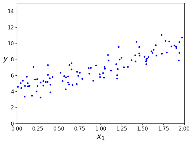
무작위 생성 선형 데이터 셋

import numpy as np

X=2*np.random.rand(100, 1)
y=4 + 3*X + np.random.randn(100, 1)

plt.plot(X, y, 'b.')
plt.xlabel('$x_1$', fontsize=18)
plt.ylabel('$y$', rotation=0, fontsize=18)
plt.axis([0,2,0,15])
save_fig("generated_data_plot")
plt.show()

그림 저장: generated_data_plot

정규 방정식으로 \(\hat{\boldsymbol{\theta}}\) 계산

• np.linalg.inv(): 역행렬 계산, dot(): 행렬의 곱셈

X_b=np.c_[np.ones((100, 1)), X] # 모든 샘플에 x0=1 추가
theta_best=np.linalg.inv(X_b.T.dot(X_b)).dot(X_b.T).dot(y)

theta_best

array([[4.21509616],
       [2.77011339]])

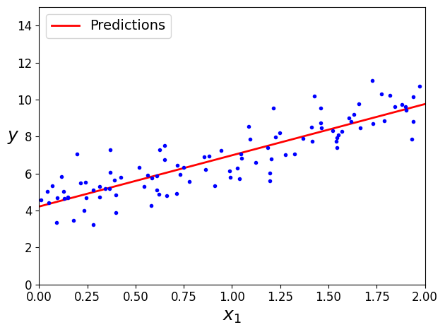
매우 비슷하지만 잡음으로 \(\boldsymbol{\theta}_0 =\) 4, \(\boldsymbol{\theta}_1 =\) 3 정확히 재현 못함

\(\hat{\boldsymbol{\theta}}\) 사용해 예측

\[\hat{y} = \mathbf{X} \boldsymbol{\hat{\theta}}\]

X_new=np.array([[0], [2]])
X_new_b=np.c_[np.ones((2,1)), X_new] # 모든 샘플에 x0=1 추가
y_predict=X_new_b.dot(theta_best)
y_predict

array([[4.21509616],
       [9.75532293]])

plt.plot(X_new, y_predict, "r-", linewidth=2, label="Predictions")
plt.plot(X, y, "b.")
plt.xlabel("$x_1$", fontsize=18)
plt.ylabel("$y$", rotation=0, fontsize=18)
plt.legend(loc="upper left", fontsize=14)
plt.axis([0, 2, 0, 15])
save_fig("linear_model_predictions_plot")
plt.show()

그림 저장: linear_model_predictions_plot

사이킷런 선형회귀 수행

• 특성의 가중치 (coef_)와 편향(intercept_)을 분리하여 저장

from sklearn.linear_model import LinearRegression

lin_reg=LinearRegression()
lin_reg.fit(X, y)
lin_reg.intercept_, lin_reg.coef_

(array([4.21509616]), array([[2.77011339]]))

lin_reg.predict(X_new)

array([[4.21509616],
       [9.75532293]])

LinearRegression 클래스는 scipy.linalg.lstsq() 함수(“least squares”의 약자)를 사용하므로 이 함수를 직접 사용할 수 있습니다:

# 싸이파이 lstsq() 함수를 사용하려면 scipy.linalg.lstsq(X_b, y)와 같이 씁니다.
theta_best_svd, residuals, rank, s=np.linalg.lstsq(X_b, y, rcond=1e-6)
theta_best_svd

array([[4.21509616],
       [2.77011339]])

이 함수는 \(\mathbf{X}^+\mathbf{y}\)을 계산합니다. \(\mathbf{X}^{+}\)는 \(\mathbf{X}\)의 유사역행렬 (pseudoinverse)입니다(Moore–Penrose 유사역행렬입니다). np.linalg.pinv()을 사용해서 유사역행렬을 직접 계산할 수 있습니다: \[\boldsymbol{\hat{\theta}} = \mathbf{X}^{-1}\hat{y}\]

np.linalg.pinv(X_b).dot(y)

array([[4.21509616],
       [2.77011339]])

유사역행렬 자체는 특이값 분해(SVD)라 부르는 표준 행렬 분해 기법을 사용해 계산

• 훈련 세트 행렬 X를 3개의 행렬 곱셈 \(\mathbf{U}\sum\mathbf{V}^{T}\) 로 분해 (numpy.linalg.svd() 참고)
• 유사역행렬 \(\mathbf{X}^{+}=\mathbf{V}\sum^{+}\mathbf{U}^{T}\) 로 계산
  1. \(\sum^{+}\) 를 계산하기 위해 \(\sum\) 을 먼저 구하고 어떤 낮은 임곗값보다 작은 모든 수를 0으로 바꿈
  2. 0이 아닌 모든 값을 역수로 치환 후, 만들어진 행렬 전치
• 정규 방정식보다 효율적이고 극단적인 경우도 처리 가능

실제로 \(m<n\) 이거나 어떤 특성이 중복되어 행렬 \(\mathbf{X}^{T}\mathbf{X}\) 의 역행렬이 없다면(즉, 특이 행렬) 정규 방정식 작동 X => 하지만, 유사역행렬은 항상 구할 수 있음

4.1.2 계산 복잡도

• 정규 방정식 \((n+1) \times (n+1)\) 크기가 되는 \(\mathbf{X}^T \mathbf{X}\) 의 역행렬 계산 (\(n\)은 특성의 수)
  • 역행렬 계산 복잡도: \(O(n^{2.4})\) ~ \(O(n^{3})\) -> 특성의 수 2배 늘어나면 계산 시간 대략 8배 늘어남
• 사이킷런의 LinearRegression 클래스가 사용하는 SVD : \(O(n^{2})\)

CAUTION
정규 방정식, SVD 모두 훈련 샘플 수에 대해서는 선형적으로 증가

• (정규 방정식이나 다른 알고리즘으로) 학습된 선형 모델 예측 계산 복잡도 선형

• 특성이 많고 훈련 샘플이 너무 많아 메모리에 담을 수 없을 때 다음의 방법 사용

4.2 경사 하강법

• 여러 종류의 문제에서 최적의 해법을 찾는 일반적인 최적화 알고리즘
• 비용 함수를 최소화하기 위해 반복해서 파라미터 조정
  • 파라미터 \(\boldsymbol{\theta}\) 에 대해 비용 함수의 현재 gradient를 계산하여 그 값이 감소하는 방향으로 진행
  • gradient가 0이 되면 최솟값에 도달한 것
  • 학습률(learning rate): 학습 스텝의 크기 (비용 함수 기울기에 비례)
    • 학습률에 따라 알고리즘 수렴을 위한 시간 결정
• 선형 회귀를 위한 MSE 함수는 볼록 함수(convex function)
  • 지역 최솟값(local minimum)이 없고, 전역 최솟값(global minimum)만 있음
  • 연속된 함수이고, 기울기가 갑자기 변하지 않음
  • 위의 두 사실로 경사 하강법이 전역 최솟값에 가깝게 접근할 수 있음을 보장 (학습률이 너무 높지 않고 충분한 시간이 주어지면)
• 특성 스케일링이 필요

CAUTION
사이킷런의 StandardScaler와 같이 모든 특성이 같은 스케일 갖도록 해야함 (그렇지 않으면 수렴 시간 오래걸림)

• 모델 훈련: (훈련 세트에서) 비용 함수를 최소화하는 모델 파라미터의 조합을 찾는 일 (모델의 파라미터 공간(parameter space)에서 찾는다)

4.2.1 배치 경사 하강법

• 각 모델 파라미터 \(\boldsymbol{\theta}_j\) 에 대해 비용 함수의 gradient를 계산 -> 편도 함수(partial derivative)

• 비용 함수의 gradient 벡터 \[\dfrac{\partial}{\partial \boldsymbol{\theta}} \text{MSE}(\boldsymbol{\theta}) = \dfrac{2}{m} \mathbf{X}^T (\mathbf{X} \boldsymbol{\theta} - \mathbf{y})\]

CAUTION

• 매 경사 하강법 스텝에서 전체 훈련 세트에 대해 계산
• 매우 큰 훈련 세트에서는 아주 느리다
• 특성 수가 엄청 많을 때는 정규방정식, SVD 보다 훨씬 빠르다

• 경사 하강법의 스텝 \[\boldsymbol{\theta}^{(\text{next step})} = \boldsymbol{\theta} - \eta \dfrac{\partial}{\partial \boldsymbol{\theta}} \text{MSE}(\boldsymbol{\theta})\]

eta=0.1 # 학습률
n_iterations=1000
m=100

theta=np.random.randn(2,1) # 랜덤 초기화

for iteration in range(n_iterations):
    gradients= 2/m * X_b.T.dot(X_b.dot(theta) - y)
    theta = theta - eta*gradients

theta

array([[4.21509616],
       [2.77011339]])

X_new_b.dot(theta)

array([[4.21509616],
       [9.75532293]])

여러가지 학습률에 따른 경사 하강법

theta_path_bgd=[]

def plot_gradient_descent(theta, eta, theta_path=None):
    m=len(X_b)
    plt.plot(X, y, 'b.')
    n_iterations=1000
    for iteration in range(n_iterations):
        if iteration<10:
            y_predict=X_new_b.dot(theta)
            style='b-' if iteration>0 else 'r--'
            plt.plot(X_new, y_predict, style)
        gradients= 2/m * X_b.T.dot(X_b.dot(theta) - y)
        theta = theta - eta*gradients
        if theta_path is not None:
            theta_path.append(theta)
    plt.xlabel('$x_1$', fontsize=18)
    plt.axis([0,2,0,15])
    plt.title(r"$\eta = {}$".format(eta), fontsize=16)

np.random.seed(42)
theta = np.random.randn(2,1)  # random initialization

plt.figure(figsize=(10,4))
plt.subplot(131); plot_gradient_descent(theta, eta=0.02)
plt.ylabel("$y$", rotation=0, fontsize=18)
plt.subplot(132); plot_gradient_descent(theta, eta=0.1, theta_path=theta_path_bgd)
plt.subplot(133); plot_gradient_descent(theta, eta=0.5)

save_fig("gradient_descent_plot")
plt.show()

그림 저장: gradient_descent_plot

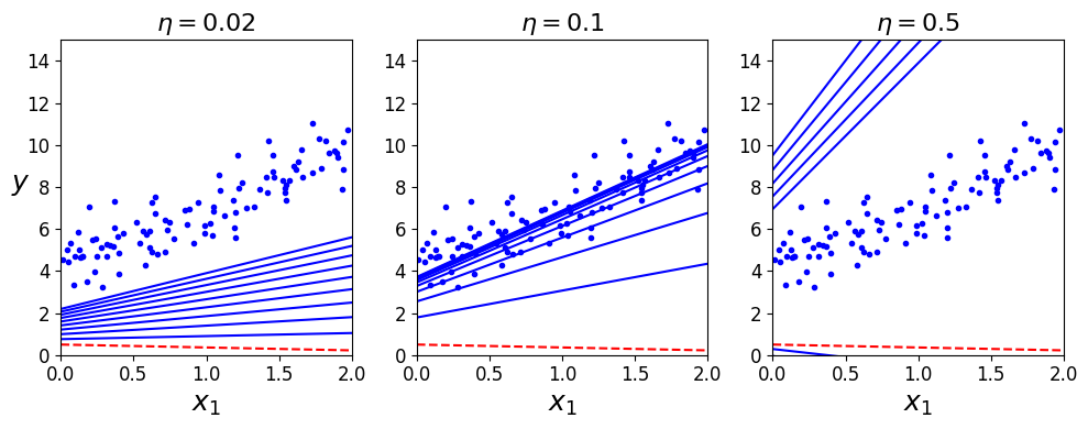
• 적절한 학습률은 그리드 탐색을 통해 찾을 수 있음 -> 수렴까지 오래걸리는 것을 막기 위해 반복 횟수 제한해야함
• 간단 해결책: 반복 횟수 아주 크게, gradient 벡터 아주 작아지면(즉, 허용오차(\(\varepsilon\))보다 작아지면) 알고리즘 중지

  수렴율

  • \(\varepsilon\) 범위 안에서 최적의 솔루셔 도달까지 \(O(1/\varepsilon)\) 의 반복이 걸릴 수 있다.
  • 즉, 허용 오차 \(\varepsilon\) 를 1/10으로 줄이면 알고리즘의 반복 10배 늘어남

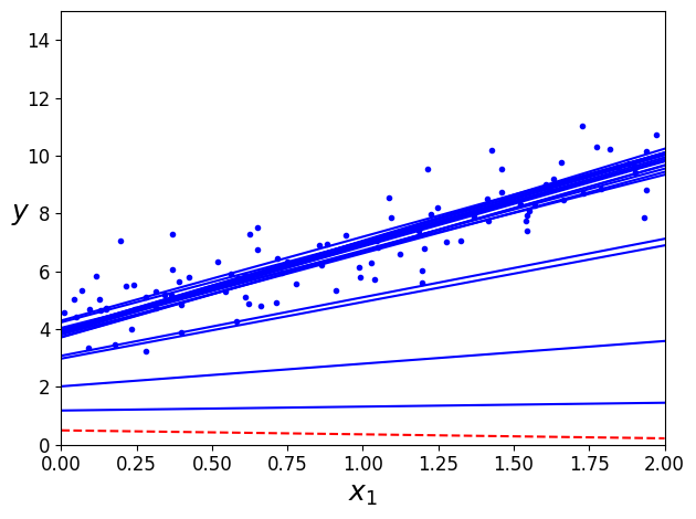
4.2.2 확률적 경사 하강법

• 배치 경사 하강법과 달리 매 스텝 한개의 샘플 무작위 선택하여 그 샘플에 대한 gradient를 계산
• 알고리즘 수행 속도 빠르고, 매우 큰 훈련 세트에서도 훈련 가능 (SGD는 외부 메모리 학습 알고리즘으로 구현 가능)
• 확률적이므로, 배치 경사 하강법보다 불안정 (요동치면서 평균적으로 감소)
  • 비용 함수가 매우 불규칙 할 때는 지역 최솟값을 건너뛰므로 배치 경사보다 좋음
  • 전역 최솟값에 다다르기 힘들다
• 학습률 감소로 해결
  • 시작할 때 크게, 점차 작게하여 전역 최솟값에 도달하게 함
  • 담금질 기법 알고리즘과 유사
  • 학습 스케줄 (learning schedule): 매 반복에서 학습률 결정하는 함수

theta_path_sgd=[]
m=len(X_b)
np.random.seed(42)

n_epochs = 50
t0, t1 = 5, 50  # 학습 스케줄 하이퍼파라미터

def learning_schedule(t):
    return t0 / (t + t1)

theta = np.random.randn(2,1)  # 랜덤 초기화

for epoch in range(n_epochs):
    for i in range(m):
        if epoch == 0 and i < 20:                    # 책에는 없음
            y_predict = X_new_b.dot(theta)           # 책에는 없음
            style = "b-" if i > 0 else "r--"         # 책에는 없음
            plt.plot(X_new, y_predict, style)        # 책에는 없음
        random_index = np.random.randint(m)
        xi = X_b[random_index:random_index+1]
        yi = y[random_index:random_index+1]
        gradients = 2 * xi.T.dot(xi.dot(theta) - yi)
        eta = learning_schedule(epoch * m + i)
        theta = theta - eta * gradients
        theta_path_sgd.append(theta)                 # 책에는 없음

plt.plot(X, y, "b.")                                 # 책에는 없음
plt.xlabel("$x_1$", fontsize=18)                     # 책에는 없음
plt.ylabel("$y$", rotation=0, fontsize=18)           # 책에는 없음
plt.axis([0, 2, 0, 15])                              # 책에는 없음
save_fig("sgd_plot")                                 # 책에는 없음
plt.show()                                           # 책에는 없음

그림 저장: sgd_plot

theta

array([[4.21076011],
       [2.74856079]])

• 샘플을 무작위로 선택 -> 샘플에 따라서 한 에포크마다 선택되는 횟수가 다르다
• 훈련 세트를 섞은 후 (입력 특성과 레이블을 동일하게 섞어야 함), 차례대로 하나씩 선택하고 다음 에포크에서 다시 섞는 방법을 사용하면 에포크마다 모든 샘플을 사용할 수 있다 (SGDRegressor, SGDClassifier의 방식) -> 보통 더 늦게 수렴한다

  CAUTION

  • 확률적 하강법 사용 시 IID(independent and identically distributed)를 만족해야 평균적으로 파라미터가 전역 최적점으로 향한다고 보장 가능
  • 훈련 동안 샘플을 섞는 것으로 위와 같이 만들 수 있다
  • 레이블 순서대로 샘플이 정렬되지 않는다면 최적점에 가깝게 도달 못함

사이킷런 SGD 방식 선형회귀 SGDRegressor 클래스

• 최대 1000번 에포크 동안 반복 (max_iter=1000)
• 한 에포크에서 0.001보다 적게 손실이 줄어들 때까지 실행 (tol=1e-3)
• 학습률 0.1(eta0=0.1)로 기본 학습 스케줄(이전과 다름) 사용

from sklearn.linear_model import SGDRegressor

sgd_reg=SGDRegressor(max_iter=1000, tol=1e-3, penalty=None, eta0=0.1, random_state=42)
sgd_reg.fit(X, y.ravel())

SGDRegressor(eta0=0.1, penalty=None, random_state=42)

sgd_reg.intercept_, sgd_reg.coef_

(array([4.24365286]), array([2.8250878]))

4.2.3 미니배치 경사 하강법

• 미니배치라고 불리는 임의의 작은 샘플 세트에 대해 gradient를 계산
• 주요 장점: GPU (행렬 연산에 최적화된 하드웨어)를 사용해서 얻는 성능 향상
• 미니 배치를 어느정도 크게하면 SGD보다 덜 불규칙하다 -> 결국 SGD보다 최솟값에 더 가까이 도달
• 지역 최솟값에서 빠져나오기 더 힘들다

theta_path_mgd=[]

n_iterations=50
minibatch_size=20

np.random.seed(42)
theta = np.random.randn(2,1)  # 랜덤 초기화

t0, t1=200, 1000
def learning_schedule(t):
    return t0/(t+t1)

t=0
for epoch in range(n_iterations):
    shuffled_indices=np.random.permutation(m)
    X_b_shuffled=X_b[shuffled_indices]
    y_shuffled=y[shuffled_indices]
    for i in range(0, m, minibatch_size):
        t+=1
        xi=X_b_shuffled[i:i+minibatch_size]
        yi=y_shuffled[i:i+minibatch_size]
        gradients=2/minibatch_size*xi.T.dot(xi.dot(theta) - yi)
        eta=learning_schedule(t)
        theta=theta-eta*gradients
        theta_path_mgd.append(theta)

theta

array([[4.25214635],
       [2.7896408 ]])

theta_path_bgd=np.array(theta_path_bgd)
theta_path_sgd=np.array(theta_path_sgd)
theta_path_mgd=np.array(theta_path_mgd)

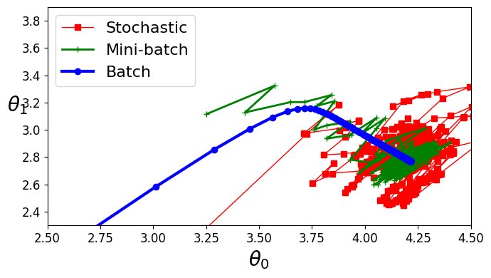
세가지 경사 하강법 알고리즘들이 훈련 과정 동안 움직인 경로 (모두 최솟값 근처에 도달)

• 배치 경사 하강법의 경로가 실제 최솟값에서 멈춤
• 미니배치, 확률적 경사 하강법은 근처에서 맴돈다
• 하지만, 배치 경사 하강법은 시간 소요가 크고 나머지 두가지도 적절한 학습 스케줄을 사용하면 최솟값에 도달한다

plt.figure(figsize=(7,4))
plt.plot(theta_path_sgd[:,0], theta_path_sgd[:, 1], 'r-s', linewidth=1, label='Stochastic')
plt.plot(theta_path_mgd[:,0], theta_path_mgd[:, 1], 'g-+', linewidth=2, label='Mini-batch')
plt.plot(theta_path_bgd[:,0], theta_path_bgd[:, 1], 'b-o', linewidth=3, label='Batch')
plt.legend(loc='upper left', fontsize=16)
plt.xlabel(r'$\theta_0$', fontsize=20)
plt.ylabel(r'$\theta_1$', fontsize=20, rotation=0)
plt.axis([2.5, 4.5, 2.3, 3.9])
save_fig("gradient_descent_paths_plot")
plt.show()

그림 저장: gradient_descent_paths_plot

선형 회귀 사용한 알고리즘 비교 (m은 샘플 수, n은 특성의 수)

알고리즘	m이 클 때	외부 메모리 지원	n이 클 때	하이퍼파라미터 수	스케일 조정 필요	사이킷런
정규 방정식	빠름	No	느림	0	No	N/A
SVD	빠름	No	느림	0	No	LinearRegression
배치 경사 하강법	느림	No	빠름	2	Yes	SGDRegressor
확률적 경사 하강법	빠름	Yes	빠름	≥2	Yes	SGDRegressor
미니배치 경사 하강법	빠름	Yes	빠름	≥2	Yes	SGDRegressor

NOTE
이 알고리즘들 훈련 결과에 차이 거의 없음 -> 모두 매우 비슷한 모델 만들고 정확히 같은 예측을 함

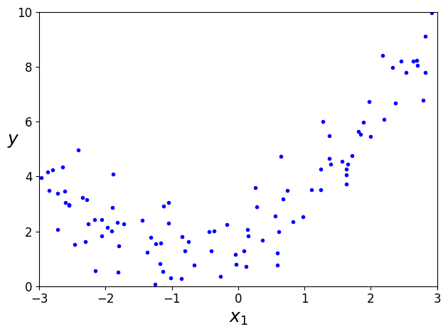
4.3 다항 회귀

• 비선형 데이터 학습 시 선형 모델 사용 가능 -> 각 특성의 거듭제곱을 새로운 특성으로 추가하고, 이 확장된 데이터 셋을 선형 모델로 훈련

import numpy as np
import numpy.random as rnd

rnd.seed(42)

# 간단한 2차방정식
m=100
X=6 * rnd.rand(m, 1) - 3
y=0.5 * X**2 + X + 2 + rnd.randn(m, 1) # 약간의 잡음 추가

plt.plot(X, y, 'b.')
plt.xlabel('$x_1$', fontsize=18)
plt.ylabel('$y$', rotation=0, fontsize=18)
plt.axis([-3, 3, 0, 10])
save_fig("quadratic_data_plot")
plt.show()

그림 저장: quadratic_data_plot

훈련 데이터 변환 -> 제곱한 새로운 특성 추가

from sklearn. preprocessing import PolynomialFeatures
poly_features=PolynomialFeatures(degree=2, include_bias=False)
X_poly=poly_features.fit_transform(X)
X[0]

array([-0.75275929])

X_poly[0]

array([-0.75275929,  0.56664654])

lin_reg=LinearRegression()
lin_reg.fit(X_poly, y)
lin_reg.intercept_, lin_reg.coef_

(array([1.78134581]), array([[0.93366893, 0.56456263]]))

X_new=np.linspace(-3,3,100).reshape(100, 1)
X_new_poly=poly_features.transform(X_new)
y_new=lin_reg.predict(X_new_poly)
plt.plot(X, y, 'b.')
plt.plot(X_new, y_new, 'r-', linewidth=2, label='Prediction')
plt.xlabel('$x_1$', fontsize=18)
plt.ylabel('$y$', rotation=0, fontsize=18)
plt.legend(loc='upper left', fontsize=14)
plt.axis([-3,3,0,10])
save_fig("quadratic_predictions_plot")
plt.show()

그림 저장: quadratic_predictions_plot

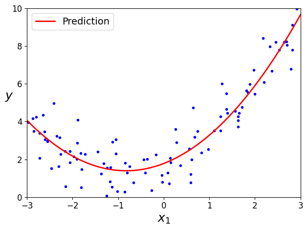
• 실제: \(\hat{y}= 0.5x_1^{2}+1.0x+2.0\)
• 예측: \(\hat{y}= 0.56x_1^{2}+0.93x+1.78\)

• 특성이 여러개일 때 다항회귀는 이 특성 사이의 관계 찾을 수 있음 (일반적인 선형 모델 불가능) => PolynomialFeatures가 주어진 차수까지 특성간의 모든 교차항 추가하기 때문
• ex) 두개의 특성 \((a, b)\), degree=3 => \(a^{2}, a^{3}, b^{2}, b^{3}, ab, ab^{2}, a^{2}b\) 특성으로 추가

CAUTION
PolynomialFeatures가(degree=d)는 특성이 n개인 배열을 특성이 \(\frac{(n+d)!}{d!n!}\) 개인 배열로 변환 => 특성 수가 교차항을 포함해 엄청 늘어남에 주의

from sklearn.preprocessing import StandardScaler
from sklearn.pipeline import Pipeline

for style, width, degree in (("g-", 1, 300), ("b--", 2, 2), ("r-+", 2, 1)):
    polybig_features = PolynomialFeatures(degree=degree, include_bias=False)
    std_scaler = StandardScaler()
    lin_reg = LinearRegression()
    polynomial_regression = Pipeline([
            ("poly_features", polybig_features),
            ("std_scaler", std_scaler),
            ("lin_reg", lin_reg),
        ])
    polynomial_regression.fit(X, y)
    y_newbig = polynomial_regression.predict(X_new)
    plt.plot(X_new, y_newbig, style, label=str(degree), linewidth=width)

plt.plot(X, y, "b.", linewidth=3)
plt.legend(loc="upper left")
plt.xlabel("$x_1$", fontsize=18)
plt.ylabel("$y$", rotation=0, fontsize=18)
plt.axis([-3, 3, 0, 10])
save_fig("high_degree_polynomials_plot")
plt.show()

그림 저장: high_degree_polynomials_plot

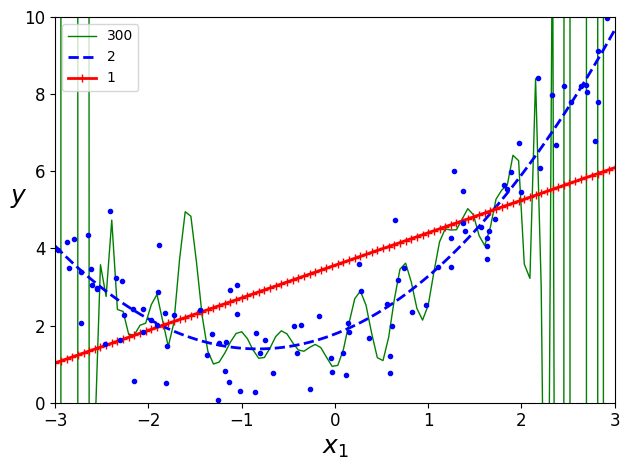
4.4 학습 곡선

• 위의 그래프: 고차 다항 회귀모델 과대적합, 선형 모델 과소적합
• 모델의 과대적합 or 과소적합 유무 확인 방법
  1. 교차 검증
     • 과대적합: 훈련데이터 성능 좋지만, 교차검증에서 나쁨 / 과소적합: 둘다 나쁨 (모델 너무 단순)
  2. 학습 곡선
     • 훈련 세트와 검증 세트 모델 성능을 훈련 세트 크기의 함수로 나타냄
     • 훈련 세트에서 크기가 다른 서브 세트를 만들어 모델을 여러번 훈련시킴

from sklearn.metrics import mean_squared_error
from sklearn.model_selection import train_test_split

def plot_learning_curves(model, X, y):
    X_train, X_val, y_train, y_val = train_test_split(X, y, test_size=0.2, random_state=10)
    train_errors, val_errors = [], []
    for m in range(1, len(X_train) + 1):
        model.fit(X_train[:m], y_train[:m])
        y_train_predict = model.predict(X_train[:m])
        y_val_predict = model.predict(X_val)
        train_errors.append(mean_squared_error(y_train[:m], y_train_predict))
        val_errors.append(mean_squared_error(y_val, y_val_predict))
        
    plt.plot(np.sqrt(train_errors), 'r-+', linewidth=2, label='train')
    plt.plot(np.sqrt(val_errors), 'b-', linewidth=3, label='val')
    plt.legend(loc='upper left', fontsize=14)
    plt.xlabel("Training set size", fontsize=14)
    plt.ylabel("RMSE", fontsize=14)  

단순 선형 회귀 모델(직선)의 학습 곡선

lin_reg=LinearRegression()
plot_learning_curves(lin_reg, X, y)
plt.axis([0, 80, 0, 3])
save_fig("underfitting_learning_curves_plot")
plt.show() 

그림 저장: underfitting_learning_curves_plot

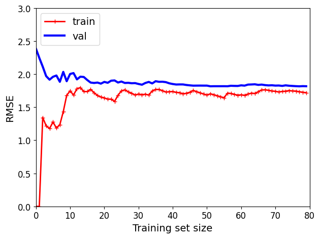
• 훈련 데이터: 샘플 수가 적을 때는 잘 작동하다가 샘플이 추가됨에 따라 완벽히 학습 불가능 => 샘플이 추가되어도 평균 오차가 크게 좋거나 나빠지지 않는다
• 검증 데이터: 적은 수의 샘플에서는 일반화되지 않아 오차가 매우 크다가 샘플이 추가됨에 따라 학습이 되고 검증 오차가 천천히 감소 => 선형 회귀는 데이터를 잘 모델링하지 못해 훈련세트의 그래프와 가까워짐
• 이 학습 곡선은 과소적합 모델의 전형적인 모습 (두 곡선이 수평한 구간 만들고 꽤 높은 오차에서 매우 가까이 근접)

TIP

• 모델이 훈련데이터에 과소적합 => 샘플 추가해도 효과 X

• 더 복잡한 모델 사용 or 더 나은 특성 활용해야함

10차 다항 회귀 모델의 학습 곡선

from sklearn.pipeline import Pipeline

polynomial_regression = Pipeline([
        ("poly_features", PolynomialFeatures(degree=10, include_bias=False)),
        ("lin_reg", LinearRegression()),
    ])

plot_learning_curves(polynomial_regression, X, y)
plt.axis([0, 80, 0, 3])           
save_fig("learning_curves_plot")
plt.show()

그림 저장: learning_curves_plot

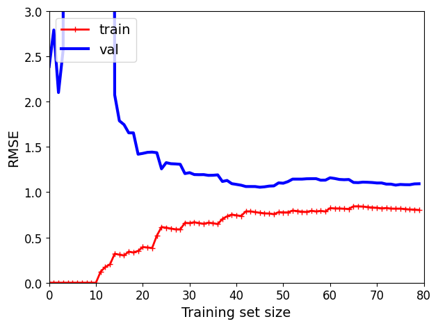
이전과 비슷해 보이지만 두 가지 매우 중요한 차이점 존재

1. 훈련 데이터의 오차가 선형 회귀 모델보다 훨씬 낮음
2. 두 곡선 사이에 공간이 있다 (훈련 데이터의 성능 > 검증 데이터의 성능) => 과대적합 모델의 특징 (더 큰 훈련 세트 사용하면 두 곡선이 점점 가까워짐)

TIP

과대적합 모델 개선 방법: 검증 오차가 훈련 오차에 접근할 때까지 더 많은 훈련 데이터 추가하는 것

편향/분산 트레이드 오프 모델의 일반화 오차는 세가지 다른 종류의 오차의 합으로 표현 가능

• 편향: 일반화 오차 중에서 잘못된 가정으로 일어난 것
  • ex) 실제 데이터가 2차인데 선형으로 가정한 경우
  • 편향이 크면 과소적합되기 쉬움
  • 선형데이터의 편향과 다른것 (여기서의 편향은 항상 분산과 같이 사용된다)
• 분산 (variance): 훈련 데이터에 있는 작은 변동에 모델이 과도하게 민감하기 때문에 나타남
  • 자유도가 높은 모델(ex> 고차 다항 회귀 모델)이 높은 분산을 가지기 쉬워 => 과대적합되기 쉽다
• 줄일 수 없는 오차 (irreducible erro): 데이터 자체에 있는 잡음 때문에 발생
  • 이 오차를 줄이는 유일한 방법: 데이터에서 잡음 제거하는 것 (ex> 고장난 센서 같은 데이터 소스를 고치거나 이상치 제거)

모델의 복잡도 커지면 분산 늘어나고 편향 줄어들음, 반대면 편향이 커지고 분산이 작아짐 => 트레이드 오프

4.5 규제가 있는 선형 모델

• 과대적합 감소의 좋은 방법 => 모델을 규제하는 것 (모델 제한)
• 다항 회귀 모델 규제하는 간단한 방법: 다항식의 차수를 감소시키는 것

4.5.1 릿지 회귀(ridge)

• 규제가 추가된 선형회귀 버전 (규제항이 비용함수에 추가) => 학습 알고리즘을 데이터에 맞추고, 모델의 가중치가 가능한 작게 유지되도록 노력
• 규제항은 훈련동안에만 비용함수에 추가, 모델의 성능은 규제항이 없는 성능 지표로 평가

NOTE

• 일반적으로 훈련동안 사용되는 비용함수 != 테스트에서 사용되는 성능 지표
• 비용함수는 최적화를 위해 미분가능해야함, 반면 성능지표는 최종 목표에 가까워야함
• ex) 비용 함수: 로그손실, 평가: 정밀도/재현율 => 분류기

• 하이퍼파라미터 \(\alpha\) : 모델을 얼마나 많이 규제할지 조절
  • \(\alpha\) = 0이면 릿지 회귀=선형회귀
  • 아주 크면 모든 가중치가 거의 0에 가까워지고 데이터의 평균을 지나는 수평선이 됨

식 4-8: 릿지 회귀의 비용 함수 \[J(\boldsymbol{\theta}) = \text{MSE}(\boldsymbol{\theta}) + \alpha \dfrac{1}{2}\sum\limits_{i=1}^{n}{\theta_i}^2\]

• 편향 \(\theta_0\) 는 규제되지 않음 (i=1 부터 시작)
• \(\mathbf{w}\) 를 특성의 가중치 벡터 (\(\theta_0\) 에서 \(\theta_n\))라고 하면 규제항은 \(\frac{1}{2}\left ( \left \| \mathbf{w} \right \|_2 \right )^{2}\) (\(\mathit{l}_2\) 노름)
• 경사 하강법에 적용하려면 MSE gradient 벡터에 \(\alpha\mathbf{w}\) 를 더하면 됨

CAUTION
릿지 회귀는 입력 특성의 스케일에 민감하기에 데이터 스케일을 맞추는 것이 중요 (ex> StandardScaler), 규제가 있는 모델은 대부분 마찬가지

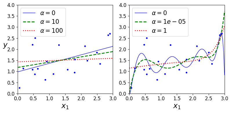
\(\alpha\) 에 따른 릿지 모델 훈련 결과 (선형 회귀와 다항 회귀)

\(\alpha\) 를 증가시킬수록 직선에 가까워짐 => 모델의 분산은 줄고 편향은 커짐

np.random.seed(42)
m=20
X=3 * np.random.rand(m, 1)
y=1 + 0.5 * X + np.random.randn(m, 1) / 1.5
X_new=np.linspace(0, 3, 100).reshape(100, 1)

from sklearn.linear_model import Ridge

def plot_model(model_class, polynomial, alphas, **model_kargs):
    for alpha, style in zip(alphas, ("b-", "g--", "r:")):
        model = model_class(alpha, **model_kargs) if alpha > 0 else LinearRegression()
        if polynomial:
            model = Pipeline([
                    ("poly_features", PolynomialFeatures(degree=10, include_bias=False)),
                    ("std_scaler", StandardScaler()),
                    ("regul_reg", model),
                ])
        model.fit(X, y)
        y_new_regul = model.predict(X_new)
        lw = 2 if alpha > 0 else 1
        plt.plot(X_new, y_new_regul, style, linewidth=lw, label=r"$\alpha = {}$".format(alpha))
    plt.plot(X, y, "b.", linewidth=3)
    plt.legend(loc="upper left", fontsize=15)
    plt.xlabel("$x_1$", fontsize=18)
    plt.axis([0, 3, 0, 4])

plt.figure(figsize=(8,4))
plt.subplot(121)
plot_model(Ridge, polynomial=False, alphas=(0, 10, 100), random_state=42)
plt.ylabel("$y$", rotation=0, fontsize=18)
plt.subplot(122)
plot_model(Ridge, polynomial=True, alphas=(0, 10**-5, 1), random_state=42)

save_fig("ridge_regression_plot")
plt.show()

그림 저장: ridge_regression_plot

선형 회귀와 마찬가지로 릿지 회귀 계산을 위해 정규 방정식 or 경사 하강법 사용 가능

사이킷런에서 정규방정식을 사용한 릿지 회귀

from sklearn.linear_model import Ridge
ridge_reg=Ridge(alpha=1, solver='cholesky', random_state=42)
ridge_reg.fit(X, y)
ridge_reg.predict([[1.5]])

array([[1.55071465]])

확률적 평균 경사 하강법 사용했을 때

• 확률적 경사 하강법과 거의 비슷하지만 현재 grdient와 이전 스텝에서 구한 모든 grdient를 합해서 평균 값으로 모델 파라미터 갱신

ridge_reg = Ridge(alpha=1, solver="sag", random_state=42) # 확률적 평균 경사 하강법
ridge_reg.fit(X, y)
ridge_reg.predict([[1.5]])

array([[1.5507201]])

확률적 경사 하강법 사용했을 때

노트: 향후 버전이 바뀌더라도 동일한 결과를 만들기 위해 사이킷런 0.21 버전의 기본값인 max_iter=1000과 tol=1e-3으로 지정

sgd_reg = SGDRegressor(penalty="l2", max_iter=1000, tol=1e-3, random_state=42)
sgd_reg.fit(X, y.ravel())
sgd_reg.predict([[1.5]])

array([1.47012588])

4.5.2 라쏘 회귀(Lasso)

• 릿지 회귀처럼 비용 함수에 규제항 더함 (규제항: 가중치 벡터의 \(\mathit{l}_1\) 노름)

식 4-10: 라쏘 회귀의 비용 함수 \[J(\boldsymbol{\theta}) = \text{MSE}(\boldsymbol{\theta}) + \alpha \sum\limits_{i=1}^{n}\left| \theta_i \right|\]

from sklearn.linear_model import Lasso

plt.figure(figsize=(8, 4))
plt.subplot(121)
plot_model(Lasso, polynomial=False, alphas=(0, 0.1, 1), random_state=42)
plt.ylabel('$y$', rotation=0, fontsize=18)
plt.subplot(122)
plot_model(Lasso, polynomial=True, alphas=(0, 10**-7, 1), random_state=42)

save_fig("lasso_regression_plot")
plt.show()

C:\Users\pjj11\anaconda3\envs\test3.7\lib\site-packages\sklearn\linear_model\_coordinate_descent.py:648: ConvergenceWarning: Objective did not converge. You might want to increase the number of iterations, check the scale of the features or consider increasing regularisation. Duality gap: 2.803e+00, tolerance: 9.295e-04
  coef_, l1_reg, l2_reg, X, y, max_iter, tol, rng, random, positive


그림 저장: lasso_regression_plot

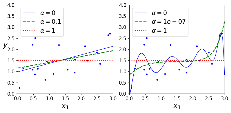
• 라쏘 회귀의 중요한 특징: 덜 중요한 특성의 가중치를 제거하려고 함 (즉, 가중치가 0이 됨) => 자동으로 특성 선택을 하고 희소 모델 (sparse model)을 만듦 (0이 아닌 특성의 가중치가 적음)

라쏘 대 릿지 규제

%matplotlib inline
import matplotlib.pyplot as plt
import numpy as np

t1a, t1b, t2a, t2b = -1, 3, -1.5, 1.5

t1s = np.linspace(t1a, t1b, 500)
t2s = np.linspace(t2a, t2b, 500)
t1, t2 = np.meshgrid(t1s, t2s)
T = np.c_[t1.ravel(), t2.ravel()]
Xr = np.array([[1, 1], [1, -1], [1, 0.5]])
yr = 2 * Xr[:, :1] + 0.5 * Xr[:, 1:]

J = (1/len(Xr) * np.sum((T.dot(Xr.T) - yr.T)**2, axis=1)).reshape(t1.shape)

N1 = np.linalg.norm(T, ord=1, axis=1).reshape(t1.shape)
N2 = np.linalg.norm(T, ord=2, axis=1).reshape(t1.shape)

t_min_idx = np.unravel_index(np.argmin(J), J.shape)
t1_min, t2_min = t1[t_min_idx], t2[t_min_idx]

t_init = np.array([[0.25], [-1]])

def bgd_path(theta, X, y, l1, l2, core = 1, eta = 0.05, n_iterations = 200):
    path = [theta]
    for iteration in range(n_iterations):
        gradients = core * 2/len(X) * X.T.dot(X.dot(theta) - y) + l1 * np.sign(theta) + l2 * theta
        theta = theta - eta * gradients
        path.append(theta)
    return np.array(path)

fig, axes = plt.subplots(2, 2, sharex=True, sharey=True, figsize=(10.1, 8))
for i, N, l1, l2, title in ((0, N1, 2., 0, "Lasso"), (1, N2, 0,  2., "Ridge")):
    JR = J + l1 * N1 + l2 * 0.5 * N2**2

    tr_min_idx = np.unravel_index(np.argmin(JR), JR.shape)
    t1r_min, t2r_min = t1[tr_min_idx], t2[tr_min_idx]

    levelsJ=(np.exp(np.linspace(0, 1, 20)) - 1) * (np.max(J) - np.min(J)) + np.min(J)
    levelsJR=(np.exp(np.linspace(0, 1, 20)) - 1) * (np.max(JR) - np.min(JR)) + np.min(JR)
    levelsN=np.linspace(0, np.max(N), 10)

    path_J = bgd_path(t_init, Xr, yr, l1=0, l2=0)
    path_JR = bgd_path(t_init, Xr, yr, l1, l2)
    path_N = bgd_path(np.array([[2.0], [0.5]]), Xr, yr, np.sign(l1)/3, np.sign(l2), core=0)

    ax = axes[i, 0]
    ax.grid(True)
    ax.axhline(y=0, color='k')
    ax.axvline(x=0, color='k')
    ax.contourf(t1, t2, N / 2., levels=levelsN)
    ax.plot(path_N[:, 0], path_N[:, 1], "y--")
    ax.plot(0, 0, "ys")
    ax.plot(t1_min, t2_min, "ys")
    ax.set_title(r"$\ell_{}$ penalty".format(i + 1), fontsize=16)
    ax.axis([t1a, t1b, t2a, t2b])
    if i == 1:
        ax.set_xlabel(r"$\theta_1$", fontsize=16)
    ax.set_ylabel(r"$\theta_2$", fontsize=16, rotation=0)

    ax = axes[i, 1]
    ax.grid(True)
    ax.axhline(y=0, color='k')
    ax.axvline(x=0, color='k')
    ax.contourf(t1, t2, JR, levels=levelsJR, alpha=0.9)
    ax.plot(path_JR[:, 0], path_JR[:, 1], "w-o")
    ax.plot(path_N[:, 0], path_N[:, 1], "y--")
    ax.plot(0, 0, "ys")
    ax.plot(t1_min, t2_min, "ys")
    ax.plot(t1r_min, t2r_min, "rs")
    ax.set_title(title, fontsize=16)
    ax.axis([t1a, t1b, t2a, t2b])
    if i == 1:
        ax.set_xlabel(r"$\theta_1$", fontsize=16)

save_fig("lasso_vs_ridge_plot")
plt.show()

그림 저장: lasso_vs_ridge_plot

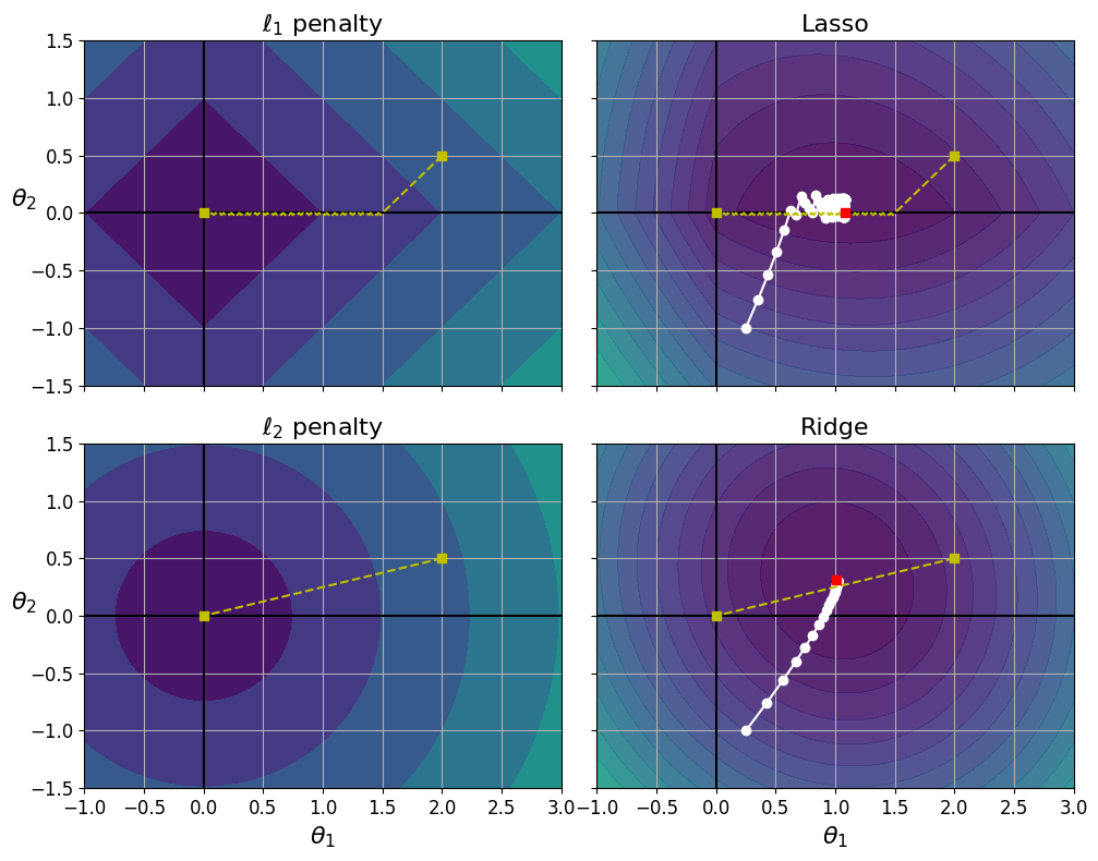
• 왼쪽 위 그래프 ( \(\mathit{l}_1\) 손실: \(\boldsymbol{\theta}_1\) 과 \(\boldsymbol{\theta}_2\) 의 절댓값의 합)
  • 축에 가까워지며 선형적으로 감소
  • \(\boldsymbol{\theta}_1=2, \boldsymbol{\theta}_2=0.5\) 로 초기화 후 시작 => \(\boldsymbol{\theta}_2\) 먼저 도달 후 \(\boldsymbol{\theta}_1\) 도달 (\(\mathit{l}_1\) 의 gradient는 0에서 정의되지 않아 진동지 조금 발생, 이 지점에서의 gradient는 -1 or 1)
• 오른쪽 위 그래프 (라쏘 손실 함수: \(\mathit{l}_1\) 손실을 더한 MSE 손실 함수)
  • 하얀 작은 원이 \(\boldsymbol{\theta}_1=0.25, \boldsymbol{\theta}_2=-1\) 로 초기화된 모델 파라미터의 최적화 과정 보여줌
  • \(\boldsymbol{\theta}_2=0\) 으로 빠르게 줄어들고 전역 최적점(빨간 사각형)에 도달
  • \(\alpha\) 가 증가하면 전역 최적점이 노란 선을 따라 왼쪽으로 이동, 감소하면 오른쪽으로 이동 (이 예에서 규제가 없는 MSE의 최적 파라미터는 \(\boldsymbol{\theta}_1=2, \boldsymbol{\theta}_2=0.5\))
• 왼쪽 아래 그래프 (\(\mathit{l}_2\) 손실)
  • 원점에 가까울수록 줄어든다 => 경사 하강법이 원점까지 직선 경로를 따라감
• 오른쪽 아래 그래프 (릿지 회귀의 비용 함수: \(\mathit{l}_2\) 손실을 더한 MSE 손실 함수)
  • 라쏘와 다른점 두가지
    1. 파라미터가 최적점에 가까워질수록 gradient가 작아짐 => 경사 하강법이 자동으로 느려져서 수렴에 도움 (진동이 없다)
    2. \(\alpha\) 를 증가시킬수록 최적의 파라미터(빨간 사각형)가 원점에 더 가까워짐 (완전히 0은 되지 않음)

TIP
라쏘를 사용할 때 최적점 근처에서 진동을 막으려면 훈련동안 점진적으로 학습률을 감소시켜야 함

• 라쏘의 비용 함수 \(\boldsymbol{\theta}_i=0 (i=1, 2, ..., n)\) 에서 미분 불가능, 하지만 \(\boldsymbol{\theta}_i=0\) 일 때, 서브그레이디언트 벡터(subgradient vector)를 사용하면 경사 하강법 적용에 문제 없음

from sklearn.linear_model import Lasso
lasso_reg=Lasso(alpha=0.1)
lasso_reg.fit(X, y)
lasso_reg.predict([[1.5]])

array([1.53788174])

Lasso 대신 SGDRegressor(penalty='l1')을 사용할 수 있음

4.5.3 엘라스틱 넷(elastic net)

• 릿지 회귀와 라쏘 회귀를 절충한 모델
• 규제항은 릿지와 라쏘의 규제항을 단순히 더해서 사용 (혼합 정도는 혼합 비율 \(r\)을 사용해 조절)

식 4-12: 엘라스틱넷 비용 함수 \[J(\boldsymbol{\theta}) = \text{MSE}(\boldsymbol{\theta}) + r \alpha \sum\limits_{i=1}^{n}\left| \theta_i \right| + \dfrac{1 - r}{2} \alpha \sum\limits_{i=1}^{n}{\theta_i}^2\]

• 사이킷런의 Lasso 클래스는 l1_ratio=1.0인 ElasticNet클래스 사용. (하지만, l1_ratio=0인 ElasticNet 과 Ridge는 다르다)

• 모델 선택 (선형 회귀(규제 X), 릿지, 라쏘, 엘라스틱넷)

  • 평번한 선형회귀는 피한다. (대부분의 경우 규제가 약간 있는것이 좋음)
  • 릿지가 기본이지만 쓰이는 특성이 몇개뿐이라고 의심되면 라쏘나 엘라스틱넷이 낫다
  • 특성 수가 훈련 샘플 수보다 많거나 특성 몇개가 강하게 연관되어 있을 때는 라쏘보다 엘라스틱넷을 선호 (라쏘는 특성 수가 샘플 수(n)보다 많으면 최대 n개의 특성 선택, 또한 여러 특성이 강하게 연관되어 있으면 이들중 임의의 특성 하나를 선택)

from sklearn.linear_model import ElasticNet
elastic_net=ElasticNet(alpha=0.1, l1_ratio=0.5, random_state=42)
elastic_net.fit(X, y)
elastic_net.predict([[1.5]])

array([1.54333232])

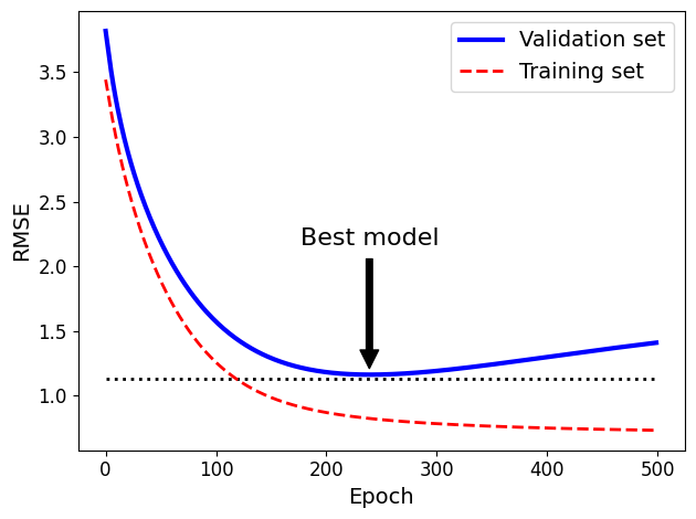
4.5.4 조기 종료

• 검증 에러가 최솟값에 도달하면 바로 훈련을 중지시키는 방법

TIP
확률적 경사 하강법, 미니배치 경사 하강법에서는 곡선이 매끄럽지 않아 최솟값 확인이 어려울 수 있음 => 검증 에러가 일정 시간 동안 최솟값보다 클 때 (모델이 더 나아지지 않는다고 확신할 때) 학습을 멈추고 검증에러가 최소일 때의 모델 파라미터로 되돌린다.

np.random.seed(42)
m=100
X=6 * np.random.rand(m, 1) - 3
y=2 + X + 0.5 * X**2 + np.random.randn(m, 1)

X_train, X_val, y_train, y_val = train_test_split(X[:50], y[:50].ravel(), test_size=0.5, random_state=10)

from copy import deepcopy

poly_scaler = Pipeline([
        ("poly_features", PolynomialFeatures(degree=90, include_bias=False)),
        ("std_scaler", StandardScaler())
    ])

X_train_poly_scaled = poly_scaler.fit_transform(X_train)
X_val_poly_scaled = poly_scaler.transform(X_val)

sgd_reg = SGDRegressor(max_iter=1, tol=None, warm_start=True, # warm_start=True로 지정하면 fit()메서드가 이전 모델 파라미터에서 훈련을 이어감
                       penalty=None, learning_rate="constant", eta0=0.0005, random_state=42)

minimum_val_error = float("inf")
best_epoch = None
best_model = None
for epoch in range(1000):
    sgd_reg.fit(X_train_poly_scaled, y_train)  # 중지된 곳에서 다시 시작
    y_val_predict = sgd_reg.predict(X_val_poly_scaled)
    val_error = mean_squared_error(y_val, y_val_predict)
    if val_error < minimum_val_error:
        minimum_val_error = val_error
        best_epoch = epoch
        best_model = deepcopy(sgd_reg)

sgd_reg = SGDRegressor(max_iter=1, tol=None, warm_start=True,
                       penalty=None, learning_rate="constant", eta0=0.0005, random_state=42)

n_epochs = 500
train_errors, val_errors = [], []
for epoch in range(n_epochs):
    sgd_reg.fit(X_train_poly_scaled, y_train)
    y_train_predict = sgd_reg.predict(X_train_poly_scaled)
    y_val_predict = sgd_reg.predict(X_val_poly_scaled)
    train_errors.append(mean_squared_error(y_train, y_train_predict))
    val_errors.append(mean_squared_error(y_val, y_val_predict))

best_epoch = np.argmin(val_errors)
best_val_rmse = np.sqrt(val_errors[best_epoch])

plt.annotate('Best model',
             xy=(best_epoch, best_val_rmse),
             xytext=(best_epoch, best_val_rmse + 1),
             ha="center",
             arrowprops=dict(facecolor='black', shrink=0.05),
             fontsize=16,
            )

best_val_rmse -= 0.03  # just to make the graph look better
plt.plot([0, n_epochs], [best_val_rmse, best_val_rmse], "k:", linewidth=2)
plt.plot(np.sqrt(val_errors), "b-", linewidth=3, label="Validation set")
plt.plot(np.sqrt(train_errors), "r--", linewidth=2, label="Training set")
plt.legend(loc="upper right", fontsize=14)
plt.xlabel("Epoch", fontsize=14)
plt.ylabel("RMSE", fontsize=14)
save_fig("early_stopping_plot")
plt.show()

그림 저장: early_stopping_plot

best_epoch, best_model

(239,
 SGDRegressor(eta0=0.0005, learning_rate='constant', max_iter=1, penalty=None,
              random_state=42, tol=None, warm_start=True))

4.6 로지스틱 회귀

• 샘플이 특정 클래스에 속할 확률을 추정하는데 널리 사용됨 => 이진 분류기

4.6.1 확률 추정

• 로지스틱 회귀 모델은 입력특성의 가중치 합 계산 + 편향 (선형 회귀 모델과 같이) => 결과값의 로지스틱(logistic) 출력
• 로지스틱: 0과 1 사이의 값을 출력하는 시그모이드 함수

t = np.linspace(-10, 10, 100)
sig = 1 / (1 + np.exp(-t))
plt.figure(figsize=(9, 3))
plt.plot([-10, 10], [0, 0], "k-")
plt.plot([-10, 10], [0.5, 0.5], "k:")
plt.plot([-10, 10], [1, 1], "k:")
plt.plot([0, 0], [-1.1, 1.1], "k-")
plt.plot(t, sig, "b-", linewidth=2, label=r"$\sigma(t) = \frac{1}{1 + e^{-t}}$")
plt.xlabel("t")
plt.legend(loc="upper left", fontsize=20)
plt.axis([-10, 10, -0.1, 1.1])
save_fig("logistic_function_plot")
plt.show()

그림 저장: logistic_function_plot

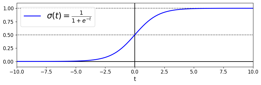
• \(t<0\) 이면 \(\sigma(t)<0.5\) 이고, \(t>0\) 이면 \(\sigma(t)>0.5\) 이므로 로지스틱 회귀 모델은 \({\boldsymbol{\theta}}^{T}\mathbf{x}\) 가 양수일 때 1(양성 클래스), 음수일 때 0(음성 클래스)이라고 예측
• 사이킷런의 LogisticRegression의 predict(), predict_proba()
  • predict(): \({\boldsymbol{\theta}}^{T}\mathbf{x}\) 값이 0보다 클 때 양성 클래스로 판단하여 결과 반환
  • predict_proba(): 시그모이드 함수를 적용하여 계산한 확률을 반환

NOTE
t (로짓(logit))

• \(logit(p)=log(1/(1-p))\) 로 정의되는 로짓함수가 로지스틱 함수의 역함수라는 사실에서 이름을 따옴
• 추정 확률 p의 로짓을 계산하면 t값 얻을 수 있음
• 양성 클래스 추정 확률과 음성 클래스 추정 확률 사이의 로그 비율이기에 로그-오즈(log-odds)라고도 불림

4.6.2 훈련과 비용 함수

• 훈련의 목적: 양성 샘플(y=1)에 대해서는 높은 확률, 음성 샘플(y=0)에 대해서는 낮은 확률을 추정하는 모델의 파라미터 벡터 \(\boldsymbol{\theta}\) 를 찾는 것

식 4-16: 하나의 훈련 샘플에 대한 비용 함수 \[c(\boldsymbol{\theta}) = \begin{cases} -\log(\hat{p}) & \text{if } y = 1, \\ -\log(1 - \hat{p}) & \text{if } y = 0. \end{cases}\]

• 샘플들을 알맞게 추정하면 비용이 0이된다.

식 4-17: 로지스틱 회귀 비용 함수(로그 손실) \[J(\boldsymbol{\theta}) = -\dfrac{1}{m} \sum\limits_{i=1}^{m}{\left[ y^{(i)} log\left(\hat{p}^{(i)}\right) + (1 - y^{(i)}) log\left(1 - \hat{p}^{(i)}\right)\right]}\]

• 모든 훈련 샘플의 비용을 평균한 것
• 이 비용함수의 최솟값을 계산하는 해는 없지만 이 함수는 볼록함수이므로 경사 하강법이 전역 최솟값을 찾는 것을 보장한다. (학습률이 너무 크지않고 충분히 기다릴 시간이 있다면)

식 4-18: 로지스틱 비용 함수의 편도 함수 \[\dfrac{\partial}{\partial \theta_j} \text{J}(\boldsymbol{\theta}) = \dfrac{1}{m}\sum\limits_{i=1}^{m}\left(\mathbf{\sigma(\boldsymbol{\theta}}^T \mathbf{x}^{(i)}) - y^{(i)}\right)\, x_j^{(i)}\]

• 식 [4-17]의 \(j\)번째 모델 파라미터 \(\boldsymbol{\theta}_j\) 에 대해 편미분 한 것
• 각 샘플에 대해 예측오차 계산하고 \(j\)번째 특성값을 곱해 모든 훈련 샘플에 대해 평균을 냄
• 모든 편도함수를 포함한 gradient 벡터를 만들면 배치 경사 하강법 사용 가능

4.6.3 결정 경계

• 붓꽃 데이터셋(iris) 활용 (3개의 품종에 속하는 붓곷 150개의 꽃잎(petal), 꽃받침(sepal)의 너비와 길이 정보)

꽃잎의 너비를 기반으로 Iris-Virginica종을 감지하는 분류기 만들기

from sklearn import datasets
iris=datasets.load_iris()
list(iris.keys())

['data',
 'target',
 'frame',
 'target_names',
 'DESCR',
 'feature_names',
 'filename',
 'data_module']

print(iris.DESCR)

.. _iris_dataset:

Iris plants dataset
--------------------

**Data Set Characteristics:**

    :Number of Instances: 150 (50 in each of three classes)
    :Number of Attributes: 4 numeric, predictive attributes and the class
    :Attribute Information:
        - sepal length in cm
        - sepal width in cm
        - petal length in cm
        - petal width in cm
        - class:
                - Iris-Setosa
                - Iris-Versicolour
                - Iris-Virginica
                
    :Summary Statistics:

    ============== ==== ==== ======= ===== ====================
                    Min  Max   Mean    SD   Class Correlation
    ============== ==== ==== ======= ===== ====================
    sepal length:   4.3  7.9   5.84   0.83    0.7826
    sepal width:    2.0  4.4   3.05   0.43   -0.4194
    petal length:   1.0  6.9   3.76   1.76    0.9490  (high!)
    petal width:    0.1  2.5   1.20   0.76    0.9565  (high!)
    ============== ==== ==== ======= ===== ====================

    :Missing Attribute Values: None
    :Class Distribution: 33.3% for each of 3 classes.
    :Creator: R.A. Fisher
    :Donor: Michael Marshall (MARSHALL%PLU@io.arc.nasa.gov)
    :Date: July, 1988

The famous Iris database, first used by Sir R.A. Fisher. The dataset is taken
from Fisher's paper. Note that it's the same as in R, but not as in the UCI
Machine Learning Repository, which has two wrong data points.

This is perhaps the best known database to be found in the
pattern recognition literature.  Fisher's paper is a classic in the field and
is referenced frequently to this day.  (See Duda & Hart, for example.)  The
data set contains 3 classes of 50 instances each, where each class refers to a
type of iris plant.  One class is linearly separable from the other 2; the
latter are NOT linearly separable from each other.

.. topic:: References

   - Fisher, R.A. "The use of multiple measurements in taxonomic problems"
     Annual Eugenics, 7, Part II, 179-188 (1936); also in "Contributions to
     Mathematical Statistics" (John Wiley, NY, 1950).
   - Duda, R.O., & Hart, P.E. (1973) Pattern Classification and Scene Analysis.
     (Q327.D83) John Wiley & Sons.  ISBN 0-471-22361-1.  See page 218.
   - Dasarathy, B.V. (1980) "Nosing Around the Neighborhood: A New System
     Structure and Classification Rule for Recognition in Partially Exposed
     Environments".  IEEE Transactions on Pattern Analysis and Machine
     Intelligence, Vol. PAMI-2, No. 1, 67-71.
   - Gates, G.W. (1972) "The Reduced Nearest Neighbor Rule".  IEEE Transactions
     on Information Theory, May 1972, 431-433.
   - See also: 1988 MLC Proceedings, 54-64.  Cheeseman et al"s AUTOCLASS II
     conceptual clustering system finds 3 classes in the data.
   - Many, many more ...

X=iris['data'][:, 3:] # 꽃잎 너비
y=(iris['target']==2).astype(int) # Iris virginica이면 1 아니면 0

노트: 향후 버전이 바뀌더라도 동일한 결과를 만들기 위해 사이킷런 0.22 버전의 기본값인 solver="lbfgs"로 지정한다.

from sklearn.linear_model import LogisticRegression
log_reg=LogisticRegression(solver='lbfgs', random_state=42)
log_reg.fit(X, y)

LogisticRegression(random_state=42)

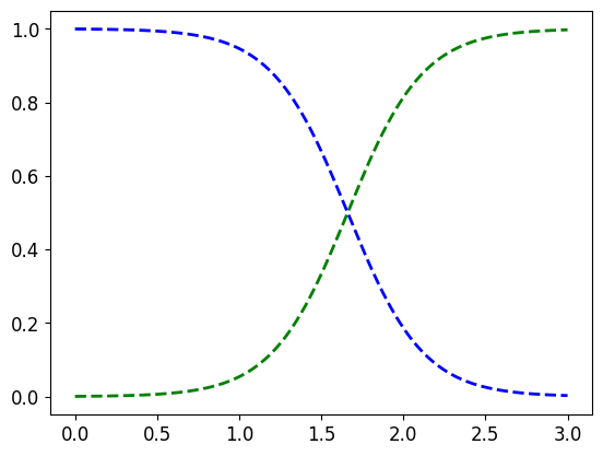
꽃잎의 너비가 0~3cm인 꽃에 대해 모델의 추정 확률 계산

X_new=np.linspace(0, 3, 1000).reshape(-1, 1) # 0~3까지의 값을 갖는 1000개의 등간격 값을 열 벡터(2D 배열)로 변환
y_proba=log_reg.predict_proba(X_new)

plt.plot(X_new, y_proba[:, 1], 'g--', linewidth=2, label='Iris virginica')
plt.plot(X_new, y_proba[:, 0], 'b--', linewidth=2, label='Not Iris virginica')

[<matplotlib.lines.Line2D at 0x2050e1e8cc8>]

책에 실린 그림은 조금 더 예쁘게 꾸몄다:

X_new = np.linspace(0, 3, 1000).reshape(-1, 1)
y_proba = log_reg.predict_proba(X_new)
decision_boundary = X_new[y_proba[:, 1] >= 0.5][0]

plt.figure(figsize=(8, 3))
plt.plot(X[y==0], y[y==0], "bs")
plt.plot(X[y==1], y[y==1], "g^")
plt.plot([decision_boundary, decision_boundary], [-1, 2], "k:", linewidth=2)
plt.plot(X_new, y_proba[:, 1], "g-", linewidth=2, label="Iris virginica")
plt.plot(X_new, y_proba[:, 0], "b--", linewidth=2, label="Not Iris virginica")
plt.text(decision_boundary+0.02, 0.15, "Decision  boundary", fontsize=14, color="k", ha="center")
plt.arrow(decision_boundary[0], 0.08, -0.3, 0, head_width=0.05, head_length=0.1, fc='b', ec='b')
plt.arrow(decision_boundary[0], 0.92, 0.3, 0, head_width=0.05, head_length=0.1, fc='g', ec='g')
plt.xlabel("Petal width (cm)", fontsize=14)
plt.ylabel("Probability", fontsize=14)
plt.legend(loc="center left", fontsize=14)
plt.axis([0, 3, -0.02, 1.02])
save_fig("logistic_regression_plot")
plt.show()

그림 저장: logistic_regression_plot

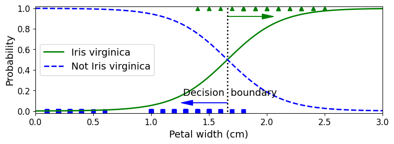
• Iris-Virginica (삼각형 표시)의 꽃잎 너비: 1.4~2.5cm에 분포
• 다른 붓꽃 (사각형 표시)의 꽃잎 너비: 0.1~1.8cm에 분포
• 꽃잎 너비 2cm 이상이면 Iris-Virginica로 강하게 확신, 1cm 아래이면 Iris-Virginica가 아니라고 강하게 확신
• 양쪽의 확률이 50%가 되는 1.6cm 근방에서 결정 경계 (decision boundary)가 만들어짐 => 꽃잎 너비 1.6cm보다 크면 Iris-Virginica, 작으면 아니라고 예측할 것이다 (아주 확실치 않더라도)

decision_boundary

array([1.66066066])

log_reg.predict([[1.7], [1.5]])

array([1, 0])

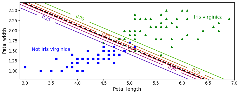
• 꽃잎 너비와 길이 두개의 특성으로 Iris-Virginica인지 확률 추정
• 점선은 모델이 50% 확률을 추정하는 지점으로 결정 경계 (이 경계는 선형)
• 15%부터 90%까지 나란한 직선들은 모델이 특정 확률을 출력하는 포인트 => 모델은 맨 오른쪽 위의 직선을 넘어서 있는 꽃들을 90% 이상의 확률로 Iris-Virginica라고 판단

from sklearn.linear_model import LogisticRegression

X = iris["data"][:, (2, 3)]  # petal length, petal width
y = (iris["target"] == 2).astype(int)

log_reg = LogisticRegression(solver="lbfgs", C=10**10, random_state=42)
log_reg.fit(X, y)

x0, x1 = np.meshgrid(
        np.linspace(2.9, 7, 500).reshape(-1, 1),
        np.linspace(0.8, 2.7, 200).reshape(-1, 1),
    )
X_new = np.c_[x0.ravel(), x1.ravel()]

y_proba = log_reg.predict_proba(X_new)

plt.figure(figsize=(10, 4))
plt.plot(X[y==0, 0], X[y==0, 1], "bs")
plt.plot(X[y==1, 0], X[y==1, 1], "g^")

zz = y_proba[:, 1].reshape(x0.shape)
contour = plt.contour(x0, x1, zz, cmap=plt.cm.brg)


left_right = np.array([2.9, 7])
boundary = -(log_reg.coef_[0][0] * left_right + log_reg.intercept_[0]) / log_reg.coef_[0][1]

plt.clabel(contour, inline=1, fontsize=12)
plt.plot(left_right, boundary, "k--", linewidth=3)
plt.text(3.5, 1.5, "Not Iris virginica", fontsize=14, color="b", ha="center")
plt.text(6.5, 2.3, "Iris virginica", fontsize=14, color="g", ha="center")
plt.xlabel("Petal length", fontsize=14)
plt.ylabel("Petal width", fontsize=14)
plt.axis([2.9, 7, 0.8, 2.7])
save_fig("logistic_regression_contour_plot")
plt.show()

그림 저장: logistic_regression_contour_plot

로지스틱 회귀 모델도 \(\mathit{l}_1, \mathit{l}_2\) 페널티 사용하여 규제 가능 (사이킷런 \(\mathit{l}_2\) 기본)

NOTE
사이킷런의 LogisticRegression 모델의 규제 강도 조절 하이퍼파라미터 (다른 선형 모델처럼) alpha 아니고, 그 역수인 C이다. (C가 높을수록 모델의 규제 줄어든다)

4.6.4 소프트맥스 회귀

• 로지스틱 회귀 모델 여러개 이진 분류기 훈련시켜 연결하지 않고 직접 다중 클래스 지원하도록 일반화 가능 => 소프트맥스 회귀(softmax regression) or 다항 로지스틱 회귀(multinomial logistic regression)
• 개념: 샘플 \(\mathbf{x}\) 가 주어지면 각 클래스 \(k\) 에 대한 점수 \(s_k(\mathbf{x})\) 를 계산하고, 그 점수에 소프트맥스 함수(정규화된 지수 함수)를 적용하여 각 클래스의 확률을 추정

• 각 클래스는 자신만의 파라미터 벡터 \(\boldsymbol{\theta}^{(k)}\) 가 있고, 이 벡터들은 파라미터 행렬(parameter matrix) \(\boldsymbol{\Theta}\) 에 저장됨

  식 4-20: 소프트맥스 함수 \[\hat{p}_k = \sigma\left(\mathbf{s}(\mathbf{x})\right)_k = \dfrac{\exp\left(s_k(\mathbf{x})\right)}{\sum\limits_{j=1}^{K}{\exp\left(s_j(\mathbf{x})\right)}}\]

  • 샘플 \(\mathbf{x}\)에 대해 각 클래스의 점수가 계산되면 소프트맥스 함수를 통과시켜 클래스 \(k\) 에 속할 확률 \(\hat{p}_k\) 추정 가능
  • \(k\) : 클래스 수
  • \(\mathbf{s}(\mathbf{x})\) : 샘플 \(\mathbf{x}\) 에 대한 각 클래스의 점수를 담은 벡터
  • \(\sigma\left(\mathbf{s}(\mathbf{x})\right)_k\) : 이 샘플이 클래스 \(k\) 에 속할 추정 확률
• 추정 확률이 가장 높은 클래스 (가장 높은 점수를 가진 클래스)를 선택 => armax 연산을 통해 \(\sigma\left(\mathbf{s}(\mathbf{x})\right)_k\) 가 최대인 \(k\) 값을 반환

TIP
소프트맥스 회귀 분류기는 한번에 하나의 클래스만 예측 (다중 출력은 아님) => 종류가 다른 붓꽃같이 상호 배타적인 클래스에서만 사용해야함 (하나의 사진에서 여러 사람의 얼굴을 인식하는 데는 사용 불가)

• 모델 훈련의 목적: 타깃 클래스에 대해서는 높은 확률을(다른 클래스에 대해서는 낮은 확률을) 추정하도록 만들기

  식 4-22: 크로스 엔트로피 비용 함수 \[J(\boldsymbol{\Theta}) = - \dfrac{1}{m}\sum\limits_{i=1}^{m}\sum\limits_{k=1}^{K}{y_k^{(i)}\log\left(\hat{p}_k^{(i)}\right)}\]

  • 크로스 엔트로피(cross entropy) 비용 함수를 최소화하는 것 => 타깃 클래스에 대해 낮은 확률을 예측하는 모델 억제 (목적에 부합)
  • 추정된 클래스의 확률이 타깃 클래스에 얼마나 잘 맞는지 측정하는 용도로도 사용
  • 이 식에서 \(y_k^{(i)}\) 는 \(i\) 번째 샘플이 클래스 \(k\) 에 속할 타깃 확률. (일반적으로 샘플이 클래스에 속하는지 아닌지에 따라 1 or 0)
  • 두 개의 클래스만 있을 때 로지스틱 회귀 비용 함수와 같다.

  식 4-23: 클래스 k에 대한 크로스 엔트로피의 그레이디언트 벡터 \[\nabla_{\boldsymbol{\theta}^{(k)}} \, J(\boldsymbol{\Theta}) = \dfrac{1}{m} \sum\limits_{i=1}^{m}{ \left ( \hat{p}^{(i)}_k - y_k^{(i)} \right ) \mathbf{x}^{(i)}}\]

  • 비용 함수의 \(\boldsymbol{\theta}^{(k)}\) 에 대한 gradient 벡터
  • 비용 함수를 최소화하기 위한 파라미터 행렬 \(\boldsymbol{\Theta}\) 를 찾기 위해 경사 하강법(또는 최적화 알고리즘) 사용 가능
• 사이킷런의 LogisticRegression 클래스가 둘 이상일 때 기본적으로 OvA(일대다) 전략 사용
• 하지만, multi_class 매개변수를 'multinomial'로 바꾸면 소프트맥스 회귀 사용 가능
• 소프트맥스 회귀 사용하려면 solver 매개변수에 'lbfgs'와 같이 소프트맥스 회귀를 지원하는 알고리즘을 지정해야함
  • L-BFGS는 BFGS 알고리즘을 제한된 메모리 공간에서 구현한것 (머신러닝 분야에서 널리 사용됨)
  • 이외에도 newton-cg, sag 매개변수가 multinomial 매개변수 지원
  • 위의 세가지 알고리즘 \(\mathit{l}_1\) 규제 지원 X
  • saga가 multinomial 과 \(\mathit{l}_1, \mathit{l}_2\) 규제를 지원하며 대규모 데이터셋에 가장 적합
• 기본적으로 하이퍼파라미터 C를 사용하여 조절 가능한 \(\mathit{l}_2\) 규제 적용

X = iris["data"][:, (2, 3)]  # 꽃잎 길이, 꽃잎 너비
y = iris["target"]

softmax_reg = LogisticRegression(multi_class="multinomial",solver="lbfgs", C=10, random_state=42)
softmax_reg.fit(X, y)

LogisticRegression(C=10, multi_class='multinomial', random_state=42)

x0, x1 = np.meshgrid(
        np.linspace(0, 8, 500).reshape(-1, 1),
        np.linspace(0, 3.5, 200).reshape(-1, 1),
    )
X_new = np.c_[x0.ravel(), x1.ravel()]


y_proba = softmax_reg.predict_proba(X_new)
y_predict = softmax_reg.predict(X_new)

zz1 = y_proba[:, 1].reshape(x0.shape)
zz = y_predict.reshape(x0.shape)

plt.figure(figsize=(10, 4))
plt.plot(X[y==2, 0], X[y==2, 1], "g^", label="Iris virginica")
plt.plot(X[y==1, 0], X[y==1, 1], "bs", label="Iris versicolor")
plt.plot(X[y==0, 0], X[y==0, 1], "yo", label="Iris setosa")

from matplotlib.colors import ListedColormap
custom_cmap = ListedColormap(['#fafab0','#9898ff','#a0faa0'])

plt.contourf(x0, x1, zz, cmap=custom_cmap)
contour = plt.contour(x0, x1, zz1, cmap=plt.cm.brg)
plt.clabel(contour, inline=1, fontsize=12)
plt.xlabel("Petal length", fontsize=14)
plt.ylabel("Petal width", fontsize=14)
plt.legend(loc="center left", fontsize=14)
plt.axis([0, 7, 0, 3.5])
save_fig("softmax_regression_contour_plot")
plt.show()

그림 저장: softmax_regression_contour_plot

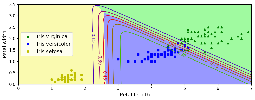
• 클래스 사이의 결정 경계가 모두 선형, Iris versicolor 클래스에 대한 확률을 곡선으로 나타냄 (0.450인 직선은 45% 확률 경계 나타냄)
• 이 모델은 추정 확률 50% 이하인 클래스 예측 가능 => 모든 결정 경계가 만나는 지점에서는 모든 클래스가 동일하게 33%의 추정 확률 가짐

softmax_reg.predict([[5, 2]])

array([2])

softmax_reg.predict_proba([[5, 2]])

array([[6.38014896e-07, 5.74929995e-02, 9.42506362e-01]])

꽃잎의 길이가 5cm, 너비가 2cm인 붓꽃 => 94.2% 확률로 Iris virginica(클래스 2) 라고 (또는 5.8% 확률로 Iris versicolor라고) 출력

출처

• 핸즈온 머신러닝 2판