5. 서포트 벡터 머신

29 Jan 2024 in ML/DL / Handson-ml2

핸즈온 머신러닝 2판에서 공부했던 내용을 정리하는 부분입니다.

SVM의 핵심 개념, 사용 방법, 작동 원리 학습

설정
5.1 선형 SVM 분류
- 5.1.1 소프트 마진 분류
5.2 비선형 SVM 분류
5.3 SVM 회귀
5.4 SVM 이론
추가 내용
- 훈련 시간
- 배치 경사 하강법을 사용한 선형 SVM 분류기 구현
연습문제 풀이
출처

설정

# 파이썬 ≥3.5 필수
import sys
assert sys.version_info >= (3, 5)

# 사이킷런 ≥0.20 필수
import sklearn
assert sklearn.__version__ >= "0.20"

# 공통 모듈 임포트
import numpy as np
import os

# 노트북 실행 결과를 동일하게 유지하기 위해
np.random.seed(42)

# 깔끔한 그래프 출력을 위해
%matplotlib inline
import matplotlib as mpl
import matplotlib.pyplot as plt
mpl.rc('axes', labelsize=14)
mpl.rc('xtick', labelsize=12)
mpl.rc('ytick', labelsize=12)

# 그림을 저장할 위치
PROJECT_ROOT_DIR = "."
CHAPTER_ID = "svm"
IMAGES_PATH = os.path.join(PROJECT_ROOT_DIR, "images", CHAPTER_ID)
os.makedirs(IMAGES_PATH, exist_ok=True)

def save_fig(fig_id, tight_layout=True, fig_extension="png", resolution=300):
    path = os.path.join(IMAGES_PATH, fig_id + "." + fig_extension)
    print("그림 저장:", fig_id)
    if tight_layout:
        plt.tight_layout()
    plt.savefig(path, format=fig_extension, dpi=resolution)

서포트 벡터 머신 (SVM)

매우 강력하고 선형이나 비선형 분류, 회귀, 이상치 탐색에도 사용 가능한 다목적 머신러닝 모델
복잡한 분류 문제에 잘 들어 맞고, 작거나 중간 크기의 데이터셋에 적합

5.1 선형 SVM 분류

<그림 5–1. 라지 마진 분류> 생성 코드

from sklearn.svm import SVC
from sklearn import datasets

iris=datasets.load_iris()
X=iris['data'][:, (2, 3)]
y=iris['target']

setosa_or_versicolor=(y==0) | (y==1)
X=X[setosa_or_versicolor]
y=y[setosa_or_versicolor]

# SVM 분류 모델
svm_clf=SVC(kernel='linear', C=float('inf'))
svm_clf.fit(X,y)

SVC(C=inf, kernel='linear')

# 나쁜 모델
x0 = np.linspace(0, 5.5, 200)
pred_1 = 5*x0 - 20
pred_2 = x0 - 1.8
pred_3 = 0.1 * x0 + 0.5

def plot_svc_decision_boundary(svm_clf, xmin, xmax):
    w = svm_clf.coef_[0]
    b = svm_clf.intercept_[0]

    # 결정 경계에서 w0*x0 + w1*x1 + b = 0 이므로
    # => x1 = -w0/w1 * x0 - b/w1
    x0 = np.linspace(xmin, xmax, 200)
    decision_boundary = -w[0]/w[1] * x0 - b/w[1]

    margin = 1/w[1]
    gutter_up = decision_boundary + margin
    gutter_down = decision_boundary - margin

    svs = svm_clf.support_vectors_
    plt.scatter(svs[:, 0], svs[:, 1], s=180, facecolors='#FFAAAA')
    plt.plot(x0, decision_boundary, "k-", linewidth=2)
    plt.plot(x0, gutter_up, "k--", linewidth=2)
    plt.plot(x0, gutter_down, "k--", linewidth=2)

fig, axes = plt.subplots(ncols=2, figsize=(10,2.7), sharey=True)

plt.sca(axes[0])
plt.plot(x0, pred_1, "g--", linewidth=2)
plt.plot(x0, pred_2, "m-", linewidth=2)
plt.plot(x0, pred_3, "r-", linewidth=2)
plt.plot(X[:, 0][y==1], X[:, 1][y==1], "bs", label="Iris versicolor")
plt.plot(X[:, 0][y==0], X[:, 1][y==0], "yo", label="Iris setosa")
plt.xlabel("Petal length", fontsize=14)
plt.ylabel("Petal width", fontsize=14)
plt.legend(loc="upper left", fontsize=14)
plt.axis([0, 5.5, 0, 2])

plt.sca(axes[1])
plot_svc_decision_boundary(svm_clf, 0, 5.5)
plt.plot(X[:, 0][y==1], X[:, 1][y==1], "bs")
plt.plot(X[:, 0][y==0], X[:, 1][y==0], "yo")
plt.xlabel("Petal length", fontsize=14)
plt.axis([0, 5.5, 0, 2])

save_fig("large_margin_classification_plot")
plt.show()

그림 저장: large_margin_classification_plot

png

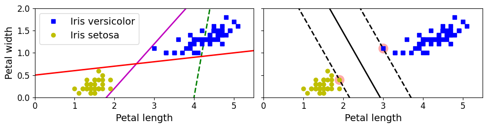
[그림 5-1]

왼쪽 그래프의 점선은 클래스 잘 분류 못하는 모델, 다른 두 모델은 훈련세트에 대해 잘 동작하지만 결정경계가 샘플에 너무 가까워서 새로운 샘플에 대해서는 잘 작동 못할 것이다
오른쪽 그래프에 있는 실선은 SVM 분류기의 결정 경계
- 두개의 클래스 분류, 제일 가까운 샘플에 대해 가능한 한 멀리 떨어져있음 => 클래스 사이의 가장 넓은 도로 찾는것 (라지 마진 분류라고 부름)
- 도로 바깥쪽에 훈련 샘플 추가해도 결정경계에 전혀 영향 미치지 않음 => 도로 경계에 위치한 샘플에의해 전적으로 결정 (서포트 벡터)

<그림 5-2. 특성 스케일에 따른 민감성> 생성 코드

Xs = np.array([[1, 50], [5, 20], [3, 80], [5, 60]]).astype(np.float64)
ys = np.array([0, 0, 1, 1])
svm_clf = SVC(kernel="linear", C=100)
svm_clf.fit(Xs, ys)

plt.figure(figsize=(9,2.7))
plt.subplot(121)
plt.plot(Xs[:, 0][ys==1], Xs[:, 1][ys==1], "bo")
plt.plot(Xs[:, 0][ys==0], Xs[:, 1][ys==0], "ms")
plot_svc_decision_boundary(svm_clf, 0, 6)
plt.xlabel("$x_0$", fontsize=20)
plt.ylabel("$x_1$    ", fontsize=20, rotation=0)
plt.title("Unscaled", fontsize=16)
plt.axis([0, 6, 0, 90])

from sklearn.preprocessing import StandardScaler
scaler = StandardScaler()
X_scaled = scaler.fit_transform(Xs)
svm_clf.fit(X_scaled, ys)

plt.subplot(122)
plt.plot(X_scaled[:, 0][ys==1], X_scaled[:, 1][ys==1], "bo")
plt.plot(X_scaled[:, 0][ys==0], X_scaled[:, 1][ys==0], "ms")
plot_svc_decision_boundary(svm_clf, -2, 2)
plt.xlabel("$x'_0$", fontsize=20)
plt.ylabel("$x'_1$  ", fontsize=20, rotation=0)
plt.title("Scaled", fontsize=16)
plt.axis([-2, 2, -2, 2])

save_fig("sensitivity_to_feature_scales_plot")

그림 저장: sensitivity_to_feature_scales_plot

png

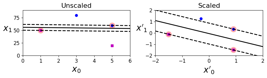
[그림 5-2]

CAUTION
SVM은 특성의 스케일에 민감, 스케일 조정 필요 (ex. 사이킷런의 StandardScaler)

5.1.1 소프트 마진 분류

<그림 5-3. 이상치에 민감한 하드 마진> 생성 코드

X_outliers = np.array([[3.4, 1.3], [3.2, 0.8]])
y_outliers = np.array([0, 0])
Xo1 = np.concatenate([X, X_outliers[:1]], axis=0)
yo1 = np.concatenate([y, y_outliers[:1]], axis=0)
Xo2 = np.concatenate([X, X_outliers[1:]], axis=0)
yo2 = np.concatenate([y, y_outliers[1:]], axis=0)

svm_clf2 = SVC(kernel="linear", C=10**9)
svm_clf2.fit(Xo2, yo2)

fig, axes = plt.subplots(ncols=2, figsize=(10,2.7), sharey=True)

plt.sca(axes[0])
plt.plot(Xo1[:, 0][yo1==1], Xo1[:, 1][yo1==1], "bs")
plt.plot(Xo1[:, 0][yo1==0], Xo1[:, 1][yo1==0], "yo")
plt.text(0.3, 1.0, "Impossible!", fontsize=24, color="red")
plt.xlabel("Petal length", fontsize=14)
plt.ylabel("Petal width", fontsize=14)
plt.annotate("Outlier",
             xy=(X_outliers[0][0], X_outliers[0][1]),
             xytext=(2.5, 1.7),
             ha="center",
             arrowprops=dict(facecolor='black', shrink=0.1),
             fontsize=16,
            )
plt.axis([0, 5.5, 0, 2])

plt.sca(axes[1])
plt.plot(Xo2[:, 0][yo2==1], Xo2[:, 1][yo2==1], "bs")
plt.plot(Xo2[:, 0][yo2==0], Xo2[:, 1][yo2==0], "yo")
plot_svc_decision_boundary(svm_clf2, 0, 5.5)
plt.xlabel("Petal length", fontsize=14)
plt.annotate("Outlier",
             xy=(X_outliers[1][0], X_outliers[1][1]),
             xytext=(3.2, 0.08),
             ha="center",
             arrowprops=dict(facecolor='black', shrink=0.1),
             fontsize=16,
            )
plt.axis([0, 5.5, 0, 2])

save_fig("sensitivity_to_outliers_plot")
plt.show()

그림 저장: sensitivity_to_outliers_plot

png

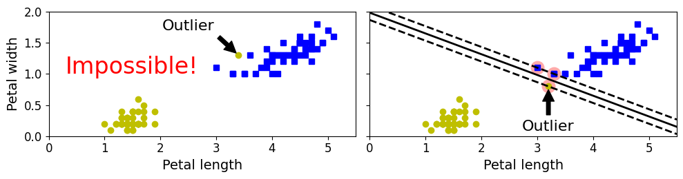
[그림 5-3]

하드 마진 분류: 모든 샘플이 도로 바깥쪽에 올바르게 분류되어 있다
- 문제점: 데이터가 선형적으로 구분 가능해야 제대로 작동, 이상치에 민감
- [그림 5-3]의 왼쪽 그래프에서 하드 마진 찾을 수 없음 (이상치 하나 있음)
- [그림 5-3]의 오른쪽 그래프 [그림 5-1]의 결정경계와 다르고 일반화 잘 안될것 같음
붓꽃 데이터 적재하고, 특성 스케일 변경, Iris-Virginia 품종을 감지하기 위해 선형 SVM 모델 훈련 (C=1과 잠시 후에 설명할 힌지 손실 함수를 적용한 LinearSVC 클래스 사용)

import numpy as np
from sklearn import datasets
from sklearn.pipeline import Pipeline
from sklearn.preprocessing import StandardScaler
from sklearn.svm import LinearSVC

iris = datasets.load_iris()
X = iris["data"][:, (2, 3)]  # 꽃잎 길이, 꽃잎 너비
y = (iris["target"] == 2).astype(np.float64)  # Iris virginica

svm_clf = Pipeline([
        ("scaler", StandardScaler()),
        ("linear_svc", LinearSVC(C=1, loss="hinge", random_state=42)),
    ])

svm_clf.fit(X, y)

Pipeline(steps=[('scaler', StandardScaler()),
                ('linear_svc', LinearSVC(C=1, loss='hinge', random_state=42))])

밑의 [그림 5-4]의 왼쪽 그래프 => 위의 코드로 만들어짐

svm_clf.predict([[5.5, 1.7]])

array([1.])

NOTE
SVM 분류기는 로지스틱 회귀 분류기와 다르게 클래스에 대한 확률 제공하지 않음 (LinearSVC 모델은 predict_proba() 메서드 제공하지 않지만, SVC 모델은 probability=True로 지정하면 predict_proba() 메서드 제공)

LinearSVC 대신 SVC, SGDClassifier 모델로 대체 가능
- SVC: SVC(kerenel='linear', C=1)
- SGDClassifier: SGDClassifier(loss='hinge', alpha=1/(m*C))
  - 선형 SVM 분류기 훈련을 위해 일반적인 확률적 경사 하강법 사용
  - LinearSVC 만큼 빠르게 수렴하지 않지만, 데이터셋이 아주 커서 메모리 적재 불가능하거나(외부 메모리 훈련), 온라인 학습으로 분류 문제 다룰 때 유용

TIP
LinearSVC는 규제에 편향 포함 시킴 => 훈련 세트에서 평균을 빼서 중앙에 맞춰야 함 (StandardScaler 사용하면 됨)
loss 매개변수 'hinge'로 지정해야 함 => LinearSVC는 보통의 SVM 구현과 다르게 규제에 편향을 포함하고 있어서 데이터 스케일을 맞추지 않고 SVC 모델과 비교하면 큰일
훈련 샘플보다 특성이 많지 않다면 성능 향상을 위해 dual 매개변수를 False로 지정해야 함 (이 장 뒷부분에서 쌍대(duality) 문제에 대해 설명)

<그림 5-4. 넓은 마진(왼쪽) 대 적은 마진 오류(오른쪽)> 생성 코드

import numpy as np
from sklearn import datasets
from sklearn.pipeline import Pipeline
from sklearn.preprocessing import StandardScaler
from sklearn.svm import LinearSVC

scaler = StandardScaler()
svm_clf1 = LinearSVC(C=1, loss="hinge", random_state=42)
svm_clf2 = LinearSVC(C=100, loss="hinge", random_state=42)

scaled_svm_clf1 = Pipeline([
        ("scaler", scaler),
        ("linear_svc", svm_clf1),
    ])
scaled_svm_clf2 = Pipeline([
        ("scaler", scaler),
        ("linear_svc", svm_clf2),
    ])

scaled_svm_clf1.fit(X, y)
scaled_svm_clf2.fit(X, y)

C:\Users\pjj11\anaconda3\envs\test3.7\lib\site-packages\sklearn\svm\_base.py:1208: ConvergenceWarning: Liblinear failed to converge, increase the number of iterations.
  ConvergenceWarning,

Pipeline(steps=[('scaler', StandardScaler()),
                ('linear_svc',
                 LinearSVC(C=100, loss='hinge', random_state=42))])

# 스케일되지 않은 파라미터로 변경
b1 = svm_clf1.decision_function([-scaler.mean_ / scaler.scale_])
b2 = svm_clf2.decision_function([-scaler.mean_ / scaler.scale_])
w1 = svm_clf1.coef_[0] / scaler.scale_
w2 = svm_clf2.coef_[0] / scaler.scale_
svm_clf1.intercept_ = np.array([b1])
svm_clf2.intercept_ = np.array([b2])
svm_clf1.coef_ = np.array([w1])
svm_clf2.coef_ = np.array([w2])

# 서포트 벡터 찾기 (libsvm과 달리 liblinear 라이브러리에서 제공하지 않기 때문에 
# LinearSVC에는 서포트 벡터가 저장되어 있지 않습니다.)
t = y * 2 - 1
support_vectors_idx1 = (t * (X.dot(w1) + b1) < 1).ravel()
support_vectors_idx2 = (t * (X.dot(w2) + b2) < 1).ravel()
svm_clf1.support_vectors_ = X[support_vectors_idx1]
svm_clf2.support_vectors_ = X[support_vectors_idx2]

fig, axes = plt.subplots(ncols=2, figsize=(10,2.7), sharey=True)

plt.sca(axes[0])
plt.plot(X[:, 0][y==1], X[:, 1][y==1], "g^", label="Iris virginica")
plt.plot(X[:, 0][y==0], X[:, 1][y==0], "bs", label="Iris versicolor")
plot_svc_decision_boundary(svm_clf1, 4, 5.9)
plt.xlabel("Petal length", fontsize=14)
plt.ylabel("Petal width", fontsize=14)
plt.legend(loc="upper left", fontsize=14)
plt.title("$C = {}$".format(svm_clf1.C), fontsize=16)
plt.axis([4, 5.9, 0.8, 2.8])

plt.sca(axes[1])
plt.plot(X[:, 0][y==1], X[:, 1][y==1], "g^")
plt.plot(X[:, 0][y==0], X[:, 1][y==0], "bs")
plot_svc_decision_boundary(svm_clf2, 4, 5.99)
plt.xlabel("Petal length", fontsize=14)
plt.title("$C = {}$".format(svm_clf2.C), fontsize=16)
plt.axis([4, 5.9, 0.8, 2.8])

save_fig("regularization_plot")

그림 저장: regularization_plot

png

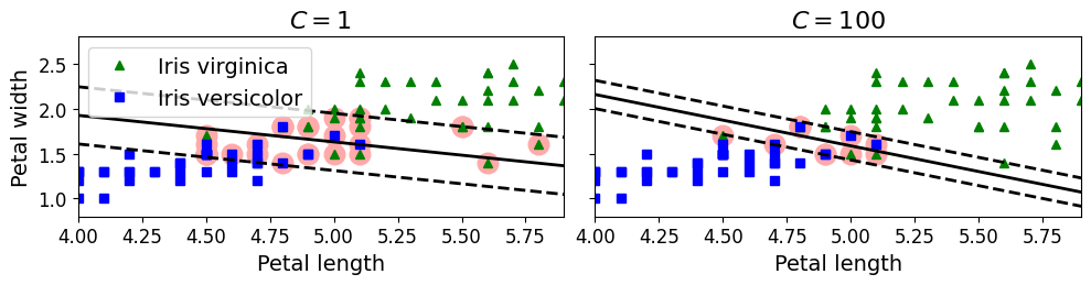
[그림 5-4]

문제 해결
- 도로의 폭을 가능한 넓게 유지하고 마진 오류(샘플이 중간 or 반대쪽에 위치) 사이에 적절한 균형이 필요 => 소프트 마진 분류
사이킷런의 SVM 모델은 여러 하이퍼파라미터 설정 가능
- C: 낮게 설정하면 왼쪽 그림과 같은 모델 생성, 높게 설정하면 오른쪽 그림과 같은 모델
- 마진 오류는 일반적으로 적은 것이 좋음 => 하지만 이 경우에는 왼쪽 모델이 일반화가 더 잘될 것 같다

TIP
SVM 모델이 과대적합이라면 C를 감소시켜서 모델 규제 가능

5.2 비선형 SVM 분류

<그림 5-5. 특성을 추가하여 선형적으로 구분되는 데이터셋 만들기>

X1D = np.linspace(-4, 4, 9).reshape(-1, 1)
X2D = np.c_[X1D, X1D**2]
y = np.array([0, 0, 1, 1, 1, 1, 1, 0, 0])

plt.figure(figsize=(10, 3))

plt.subplot(121)
plt.grid(True, which='both')
plt.axhline(y=0, color='k')
plt.plot(X1D[:, 0][y==0], np.zeros(4), "bs")
plt.plot(X1D[:, 0][y==1], np.zeros(5), "g^")
plt.gca().get_yaxis().set_ticks([])
plt.xlabel(r"$x_1$", fontsize=20)
plt.axis([-4.5, 4.5, -0.2, 0.2])

plt.subplot(122)
plt.grid(True, which='both')
plt.axhline(y=0, color='k')
plt.axvline(x=0, color='k')
plt.plot(X2D[:, 0][y==0], X2D[:, 1][y==0], "bs")
plt.plot(X2D[:, 0][y==1], X2D[:, 1][y==1], "g^")
plt.xlabel(r"$x_1$", fontsize=20)
plt.ylabel(r"$x_2$  ", fontsize=20, rotation=0)
plt.gca().get_yaxis().set_ticks([0, 4, 8, 12, 16])
plt.plot([-4.5, 4.5], [6.5, 6.5], "r--", linewidth=3)
plt.axis([-4.5, 4.5, -1, 17])

plt.subplots_adjust(right=1)

save_fig("higher_dimensions_plot", tight_layout=False)
plt.show()

그림 저장: higher_dimensions_plot

png

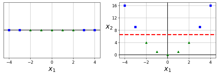
[그림 5-5]

비선형 데이터셋을 다루는 한 가지 방법 => (4장에서처럼) 다항 특성과 같은 특성 추가
- [그림 5-5]의 왼쪽 그래프 선형적 구분 안됨
- 오른쪽 그래프는 완벽하게 선형적으로 구분 가능 ($x_2=(x_1)^{2}$ 을 추가하여 만들어진 2차원 데이터셋) 구현
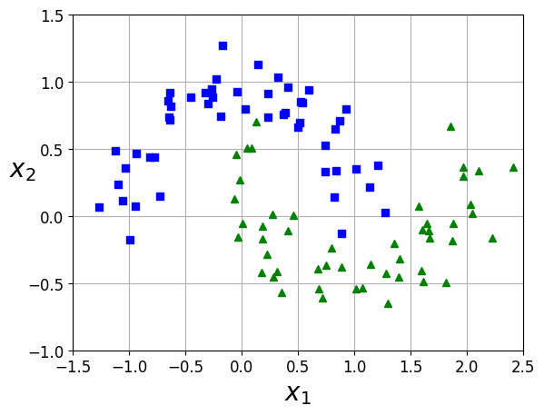
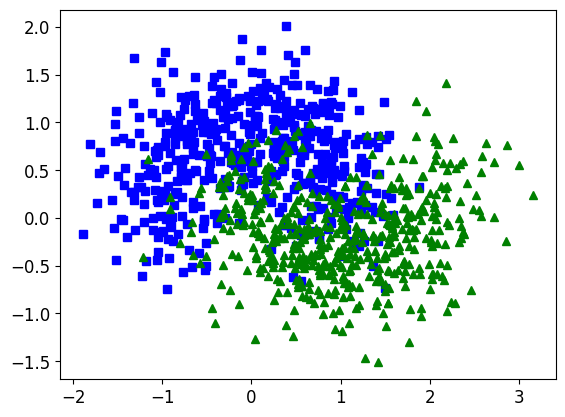
PolynomialFeatures 변환기, StandardScaler, LinearSVC 를 연결하여 Pipeline을 만듦
moons 데이터셋에 적용 (마주보는 두 개의 반원 모양으로 데이터 포인트가 놓여 있는 이진 분류를 위한 작은 데이터셋 [그림 5-6])

from sklearn.datasets import make_moons
X, y=make_moons(n_samples=100, noise=0.15, random_state=42)

def plot_dataset(X, y, axes):
    plt.plot(X[:, 0][y==0], X[:, 1][y==0], 'bs')
    plt.plot(X[:, 0][y==1], X[:, 1][y==1], 'g^')
    plt.axis(axes)
    plt.grid(True, which='both')
    plt.xlabel(r"$x_1$", fontsize=20)
    plt.ylabel(r"$x_2$", fontsize=20, rotation=0)

plot_dataset(X, y, [-1.5, 2.5, -1, 1.5])
plt.show()

png

from sklearn.datasets import make_moons
from sklearn.pipeline import Pipeline
from sklearn.preprocessing import PolynomialFeatures

polynomial_svm_clf=Pipeline([
    ('poly_features', PolynomialFeatures(degree=3)),
    ('scaler', StandardScaler()),
    ('svm_clf', LinearSVC(C=10, loss='hinge', random_state=42))
])

polynomial_svm_clf.fit(X, y)

C:\Users\pjj11\anaconda3\envs\test3.7\lib\site-packages\sklearn\svm\_base.py:1208: ConvergenceWarning: Liblinear failed to converge, increase the number of iterations.
  ConvergenceWarning,

Pipeline(steps=[('poly_features', PolynomialFeatures(degree=3)),
                ('scaler', StandardScaler()),
                ('svm_clf', LinearSVC(C=10, loss='hinge', random_state=42))])

<그림 5-6. 다항 특성을 사용한 선형 SVM 분류기> 생성 코드

def plot_predictions(clf, axes):
    x0s=np.linspace(axes[0], axes[1], 100)
    x1s=np.linspace(axes[2], axes[3], 100)
    x0, x1=np.meshgrid(x0s, x1s)
    X=np.c_[x0.ravel(), x1.ravel()]
    y_pred = clf.predict(X).reshape(x0.shape)
    y_decision = clf.decision_function(X).reshape(x0.shape)
    plt.contourf(x0, x1, y_pred, cmap=plt.cm.brg, alpha=0.2)
    plt.contourf(x0, x1, y_decision, cmap=plt.cm.brg, alpha=0.1)

plot_predictions(polynomial_svm_clf, [-1.5, 2.5, -1, 1.5])
plot_dataset(X, y, [-1.5, 2.5, -1, 1.5])

save_fig("moons_polynomial_svc_plot")
plt.show()

그림 저장: moons_polynomial_svc_plot

png

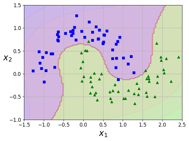
[그림 5-6]

5.2.1 다항식 커널

다항식 특성 추가는 쉽고 모든 머신러닝 알고리즘에서 잘 작동한다
- 다항식 특성 추가의 문제점
  - 낮은 차수의 다항식은 복잡한 데이터셋 잘 표현 못함
  - 높은 차수의 다항식은 많은 특성을 추가하여 모델을 느리게 만듦
커널 트릭(kernel trick): 실제 특성을 추가하지 않으면서 추가한 것과 같은 결과 얻을 수 있음
- SVC 파이썬 클래스에 구현되어있음

from sklearn.svm import SVC

poly_kernel_svm_clf=Pipeline([
    ('scaler', StandardScaler()),
    ('svm_clf', SVC(kernel='poly', degree=3, coef0=1, C=5))
])

poly_kernel_svm_clf.fit(X, y)

Pipeline(steps=[('scaler', StandardScaler()),
                ('svm_clf', SVC(C=5, coef0=1, kernel='poly'))])

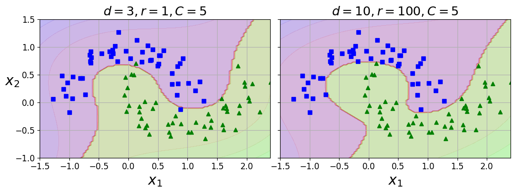
이 코드는 3차 다항식 커널을 이용하여 SVM 훈련 시킴
- 결과는 [그림 5-7]의 왼쪽
- [그림 5-7]의 오른쪽 그래프는 10차 다항식 커널을 사용한 또 다른 SVM 분류기
- 모델이 과대적합이면 다항식의 차수를 줄이고, 과소적합이면 차수를 늘린다
- 매개변수 coef0는 모델이 얼마나 차수에 영향 받을지 조절
  - coef0을 적절히 조절하면 고차항의 영향을 줄일 수 있음 (기본값: 0)

TIP
적절한 하이퍼파라미터 찾는 일반적인 방법: 그리드 탐색
처음에는 폭을 크게 하다가 세밀하게 검색해간다

<그림 5-7. 다항식 커널을 사용한 SVM 분류기> 생성 코드

poly100_kernel_svm_clf=Pipeline([
    ('scaler', StandardScaler()),
    ('svm_clf', SVC(kernel='poly', degree=10, coef0=100, C=5))
])

poly100_kernel_svm_clf.fit(X, y)

Pipeline(steps=[('scaler', StandardScaler()),
                ('svm_clf', SVC(C=5, coef0=100, degree=10, kernel='poly'))])

fig, axes = plt.subplots(ncols=2, figsize=(10.5, 4), sharey=True)

plt.sca(axes[0])
plot_predictions(poly_kernel_svm_clf, [-1.5, 2.45, -1, 1.5])
plot_dataset(X, y, [-1.5, 2.4, -1, 1.5])
plt.title(r"$d=3, r=1, C=5$", fontsize=18)

plt.sca(axes[1])
plot_predictions(poly100_kernel_svm_clf, [-1.5, 2.45, -1, 1.5])
plot_dataset(X, y, [-1.5, 2.4, -1, 1.5])
plt.title(r"$d=10, r=100, C=5$", fontsize=18)
plt.ylabel("")

save_fig("moons_kernelized_polynomial_svc_plot")
plt.show()

그림 저장: moons_kernelized_polynomial_svc_plot

png

[그림 5-7]

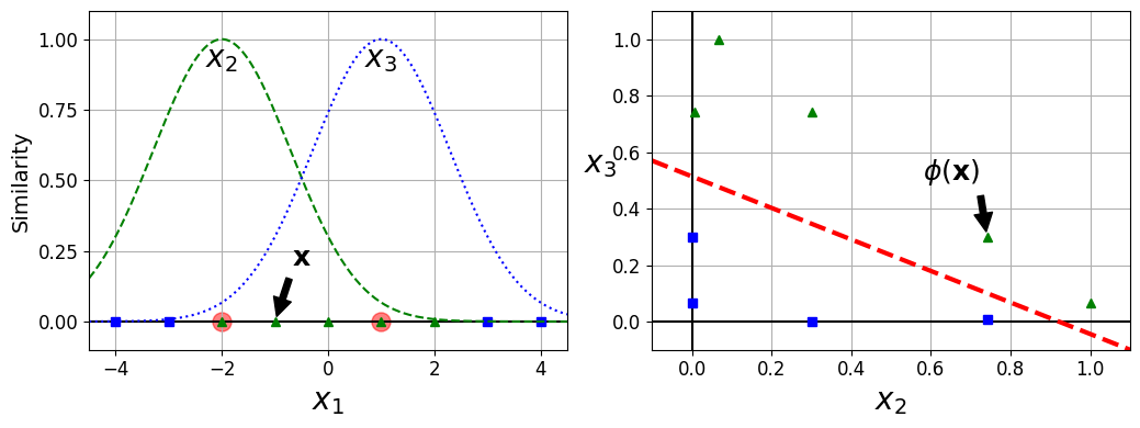
5.2.2 유사도 측정

각 샘플이 랜드마크와 얼마나 닮았는지 측정하는 유사도 함수로 계산한 특성을 추가하는 것
- 예시
  - 앞에서 본 1차원 데이터셋에 두 개의 랜드마크 $x_1=-2$ 와 $x_1=1$ 을 추가
  - $\gamma=0.3$ 인 가우시안 방사 기저 함수(RBF) 를 유사도 함수로 정의
식 5-1: 가우시안 RBF
${\displaystyle \phi_{\gamma}(\mathbf{x}, \boldsymbol{\ell})} = {\displaystyle \exp({\displaystyle -\gamma \left\| \mathbf{x} - \boldsymbol{\ell} \right\|^2})}$
- 이 함수의 값은 0~1까지 변화하며 종 모양으로 나타남 ($\gamma$ 는 0보다 커야하며 값이 작을수록 폭이 넓은 종 모양이 된다)
- [그림 5-8]의 오른쪽 그래프는 변환된 데이터셋을 보여준다(원본 특성 제외) => 이제 선형적으로 구분 가능

<그림 5-8. 가우시안 RBF를 사용한 유사도 특성> 생성 코드

def gaussian_rbf(x, landmark, gamma):
    return np.exp(-gamma * np.linalg.norm(x - landmark, axis=1)**2)

gamma = 0.3

x1s = np.linspace(-4.5, 4.5, 200).reshape(-1, 1)
x2s = gaussian_rbf(x1s, -2, gamma)
x3s = gaussian_rbf(x1s, 1, gamma)

XK = np.c_[gaussian_rbf(X1D, -2, gamma), gaussian_rbf(X1D, 1, gamma)]
yk = np.array([0, 0, 1, 1, 1, 1, 1, 0, 0])

plt.figure(figsize=(10.5, 4))

plt.subplot(121)
plt.grid(True, which='both')
plt.axhline(y=0, color='k')
plt.scatter(x=[-2, 1], y=[0, 0], s=150, alpha=0.5, c="red")
plt.plot(X1D[:, 0][yk==0], np.zeros(4), "bs")
plt.plot(X1D[:, 0][yk==1], np.zeros(5), "g^")
plt.plot(x1s, x2s, "g--")
plt.plot(x1s, x3s, "b:")
plt.gca().get_yaxis().set_ticks([0, 0.25, 0.5, 0.75, 1])
plt.xlabel(r"$x_1$", fontsize=20)
plt.ylabel(r"Similarity", fontsize=14)
plt.annotate(r'$\mathbf{x}$',
             xy=(X1D[3, 0], 0),
             xytext=(-0.5, 0.20),
             ha="center",
             arrowprops=dict(facecolor='black', shrink=0.1),
             fontsize=18,
            )
plt.text(-2, 0.9, "$x_2$", ha="center", fontsize=20)
plt.text(1, 0.9, "$x_3$", ha="center", fontsize=20)
plt.axis([-4.5, 4.5, -0.1, 1.1])

plt.subplot(122)
plt.grid(True, which='both')
plt.axhline(y=0, color='k')
plt.axvline(x=0, color='k')
plt.plot(XK[:, 0][yk==0], XK[:, 1][yk==0], "bs")
plt.plot(XK[:, 0][yk==1], XK[:, 1][yk==1], "g^")
plt.xlabel(r"$x_2$", fontsize=20)
plt.ylabel(r"$x_3$  ", fontsize=20, rotation=0)
plt.annotate(r'$\phi\left(\mathbf{x}\right)$',
             xy=(XK[3, 0], XK[3, 1]),
             xytext=(0.65, 0.50),
             ha="center",
             arrowprops=dict(facecolor='black', shrink=0.1),
             fontsize=18,
            )
plt.plot([-0.1, 1.1], [0.57, -0.1], "r--", linewidth=3)
plt.axis([-0.1, 1.1, -0.1, 1.1])
    
plt.subplots_adjust(right=1)

save_fig("kernel_method_plot")
plt.show()

그림 저장: kernel_method_plot

png

[그림 5-8]

x1_example=X1D[3, 0]
for landmark in (-2, 1):
    k=gaussian_rbf(np.array([[x1_example]]), np.array([[landmark]]), gamma)
    print('Phi({}, {}) = {}'.format(x1_example, landmark, k))

Phi(-1.0, -2) = [0.74081822]
Phi(-1.0, 1) = [0.30119421]

랜드마크 선택 방법
- 데이터셋에 있는 모든 샘플 위치에 랜드마크 설정
  - 장점: 차원이 매우 커지고, 변환된 훈련 세트가 선형적으로 구분될 가능성 높음
  - 단점: $m \times n$ 에서 $m \times m$으로 훈련 세트가 변환 됨 => 훈련 세트가 아주 크면 특성의 수가 너무 커짐(m: 샘플의 수, n: 특성의 수, 원본 특성은 제외된다고 가정)

5.2.3 가우시안 RBF 커널

유사도 특성 방식을 커널 트릭 방식으로 적용 (유사도 특성 많이 추가하는 것과 같은 비슷한 효과)

rbf_kernel_svm_clf=Pipeline([
    ('scaler', StandardScaler()),
    ('svm_clf', SVC(kernel='rbf', gamma=5, C=0.001))
])

rbf_kernel_svm_clf.fit(X, y)

Pipeline(steps=[('scaler', StandardScaler()),
                ('svm_clf', SVC(C=0.001, gamma=5))])

<그림 5-9. RBF 커널을 사용한 SVM 분류기> 생성 코드

from sklearn.svm import SVC

gamma1, gamma2 = 0.1, 5
C1, C2 = 0.001, 1000
hyperparams=(gamma1, C1),(gamma1, C2), (gamma2, C1), (gamma2, C2)

svm_clfs=[]
for gamma, C in hyperparams:
    rbf_kernel_svm_clf=Pipeline([
    ('scaler', StandardScaler()),
    ('svm_clf', SVC(kernel='rbf', gamma=gamma, C=C))
    ])
    rbf_kernel_svm_clf.fit(X, y)
    svm_clfs.append(rbf_kernel_svm_clf)

fig, axes = plt.subplots(nrows=2, ncols=2, figsize=(10.5, 7), sharex=True, sharey=True)

for i, svm_clf in enumerate(svm_clfs):
    plt.sca(axes[i // 2, i % 2])
    plot_predictions(svm_clf, [-1.5, 2.45, -1, 1.5])
    plot_dataset(X, y, [-1.5, 2.45, -1, 1.5])
    gamma, C = hyperparams[i]
    plt.title(r"$\gamma = {}, C = {}$".format(gamma, C), fontsize=16)
    if i in (0, 1):
        plt.xlabel("")
    if i in (1, 3):
        plt.ylabel("")

save_fig("moons_rbf_svc_plot")
plt.show()

그림 저장: moons_rbf_svc_plot

png

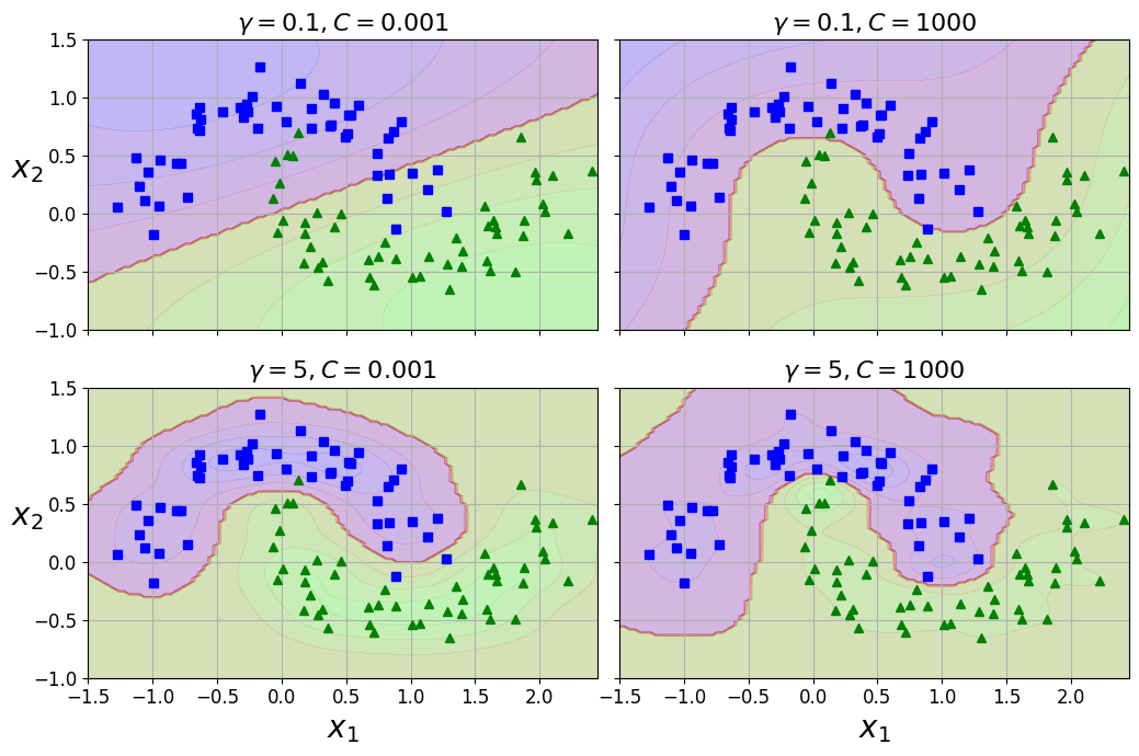
[그림 5-9]

gamma 증가: 종 모양의 그래프가 좁아져서 ([그림 5-8]의 왼쪽 그래프) 각 샘플의 영향 범위 작아짐, 결정 경계가 조금 더 불규칙해지고 샘플을 따라 구불구불 휘어짐
gamma 감소: 종 모양의 그래프 넓어지고 결정 경계가 더 부드러워짐
결국 하이퍼파라미터 $\gamma$ 가 규제의 역할 => 과대적합인 경우 감소, 과소적합인 경우 증가 (하이퍼 파라미터 C와 비슷)
- 따라서 gamma 와 C 하이퍼파라미터를 함께 조정하는 것이 좋음
다른 커널도 있지만 거의 사용되지 않음, 어떤 커널들은 데이터 구조에 특화되어 있음
- 문자열 커널 : 텍스트 문자나 DNA 서열을 분류할 때 사용됨 (ex: 문자열 서브시퀀스 커널이나 레베슈타인 거리 기반의 커널)

TIP
선형 커널을 가장 먼저 시도해봐야 한다 (LinearSVC가 SVC(kernel='linear')보다 훨씬 빠르다는 것 기억) => 특히 훈련 세트가 아주 크거나 특성 수가 많을 경우
훈련 세트가 너무 크지 않다면 RBF 커널도 시도하면 좋음 => 대부분의 경우 이 커널이 잘 맞음
시간과 컴퓨팅 성능이 좋으면 교차검증 or 그리드 탐색으로 다른 커널 시도 가능 => 특히 훈련 데이터에 특화된 커널이 있으면 테스트 수행

5.2.4 계산 복잡도

LinearSVC
- 선형 SVM을 위한 최적화된 알고리즘을 구현한 liblinear 라이브러리 기반
- 알고리즘 훈련 시간 복잡도 대략 $O(m \times n)$
정밀도 높이면 알고리즘 수행 시간 길어짐 => 허용 오차 하이퍼파라미터 $\varepsilon$으로 조절 (사이킷런에서는 매개변수 tol)
- 대부분 기본 값이면 잘 작동 (SVC의 tol기본값: 0.001, LinearSVC의 tol기본값: 0.0001)
SVC
- 커널 트릭 알고리즘을 구현한 libsvm 라이브러리 기반
- 훈련의 시간 복잡도: $O(m^{2} \times n)$ ~ $O(m^{3} \times n)$
- 훈련 샘플 수의 영향을 많이 받음 => 복잡하지만 작거나 중간 규모의 훈련 세트에 적합
- 특성의 개수에는, 특히 희소 특성(각 샘플에 0이 아닌 특성이 몇개 없는 경우) 인 경우 잘 확장 => 알고리즘의 성능이 샘플이 가진 0이 아닌 특성의 평균 수에 거의 비례

파이썬 클래스	시간 복잡도	외부 메모리 학습 지원	스케일 조정 필요성	커널 트릭
`LinearSVC`	$O(m \times n)$	아니오	예	아니오
`SGDClassifier`	$O(m \times n)$	예	예	아니오
`SVC`	$O(m^{2} \times n)$ ~ $O(m^{3} \times n)$	아니오	예	예

5.3 SVM 회귀

SVM을 분류가 아니라 회귀에 적용하는 방법: 목표를 반대로
- 일정한 마진 오류안에서 두 클래스 간의 도로 폭이 가능한 한 최대가 되도록 하는 대신, 제한된 마진 오류 (즉, 도로 밖의 샘플) 안에서 도로 안에 가능한 많은 샘플이 들어가도록 학습
- 도로의 폭은 하이퍼파라미터 $\varepsilon$ 으로 조절
  - 허용오차의 하이퍼파라미터 $\varepsilon$ 과 다름
  - SVM 회귀 모델인 SVR 과 LinearSVR 에서 허용오차는 tol 매개변수, 도로의 폭은 epsilon
  - SVR 과 LinearSVR 의 tol 매개 변수의 기본값 = SVC 과 LinearSVC 의 tol 매개 변수의 기본값 (0.001, 0.0001)

np.random.seed(42)
m=50
X=2 * np.random.rand(m, 1)
y = (4 + 3*X + np.random.randn(m, 1)).ravel()

from sklearn.svm import LinearSVR

svm_reg=LinearSVR(epsilon=1.5, random_state=42)
svm_reg.fit(X, y)

LinearSVR(epsilon=1.5, random_state=42)

<그림 5-10. SVM 회귀> 생성 코드

svm_reg1 = LinearSVR(epsilon=1.5, random_state=42)
svm_reg2 = LinearSVR(epsilon=0.5, random_state=42)
svm_reg1.fit(X, y)
svm_reg2.fit(X, y)

def find_support_vectors(svm_reg, X, y):
    y_pred = svm_reg.predict(X)
    off_margin = (np.abs(y - y_pred) >= svm_reg.epsilon)
    return np.argwhere(off_margin)

svm_reg1.support_ = find_support_vectors(svm_reg1, X, y)
svm_reg2.support_ = find_support_vectors(svm_reg2, X, y)

eps_x1 = 1
eps_y_pred = svm_reg1.predict([[eps_x1]])

def plot_svm_regression(svm_reg, X, y, axes):
    x1s = np.linspace(axes[0], axes[1], 100).reshape(100, 1)
    y_pred = svm_reg.predict(x1s)
    plt.plot(x1s, y_pred, "k-", linewidth=2, label=r"$\hat{y}$")
    plt.plot(x1s, y_pred + svm_reg.epsilon, "k--")
    plt.plot(x1s, y_pred - svm_reg.epsilon, "k--")
    plt.scatter(X[svm_reg.support_], y[svm_reg.support_], s=180, facecolors='#FFAAAA')
    plt.plot(X, y, "bo")
    plt.xlabel(r"$x_1$", fontsize=18)
    plt.legend(loc="upper left", fontsize=18)
    plt.axis(axes)

fig, axes = plt.subplots(ncols=2, figsize=(9, 4), sharey=True)
plt.sca(axes[0])
plot_svm_regression(svm_reg1, X, y, [0, 2, 3, 11])
plt.title(r"$\epsilon = {}$".format(svm_reg1.epsilon), fontsize=18)
plt.ylabel(r"$y$", fontsize=18, rotation=0)
#plt.plot([eps_x1, eps_x1], [eps_y_pred, eps_y_pred - svm_reg1.epsilon], "k-", linewidth=2)
plt.annotate(
        '', xy=(eps_x1, eps_y_pred), xycoords='data',
        xytext=(eps_x1, eps_y_pred - svm_reg1.epsilon),
        textcoords='data', arrowprops={'arrowstyle': '<->', 'linewidth': 1.5}
    )
plt.text(0.91, 5.6, r"$\epsilon$", fontsize=20)
plt.sca(axes[1])
plot_svm_regression(svm_reg2, X, y, [0, 2, 3, 11])
plt.title(r"$\epsilon = {}$".format(svm_reg2.epsilon), fontsize=18)
save_fig("svm_regression_plot")
plt.show()

그림 저장: svm_regression_plot

png

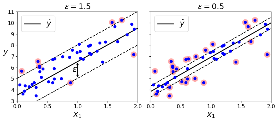
[그림 5-10]

마진 안에서 훈련 샘플이 추가되어도 모델의 예측에는 영향이 없음 => $\varepsilon$ 에 민감하지 않다 라고 함
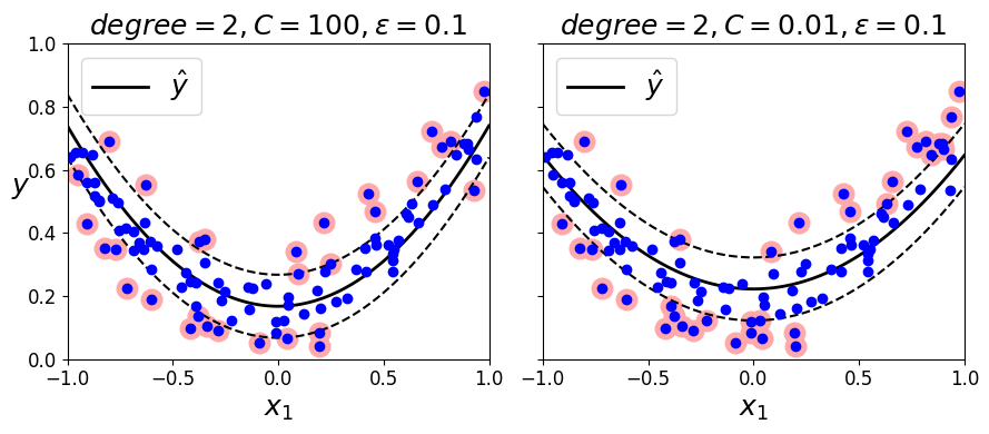
비선형 회귀 작업 처리는 커널 SVM 모델을 사용
[그림 5-11] 은 임의의 2차 방정식 형태의 훈련 세트에 2차 다항 커널을 사용한 SVM 회귀 보여줌
- 왼쪽 그래프는 규제가 거의 없고 (즉, 아주 큰 C), 오른쪽은 규제가 훨씬 많음 (즉, 작은 C)

np.random.seed(42)
m = 100
X = 2 * np.random.rand(m, 1) - 1
y = (0.2 + 0.1 * X + 0.5 * X**2 + np.random.randn(m, 1)/10).ravel()

노트: 향후 버전을 위해 사이킷런 0.22에서 기본값이 될 gamma="scale"으로 지정

from sklearn.svm import SVR

svm_poly_reg = SVR(kernel="poly", degree=2, C=100, epsilon=0.1, gamma="scale")
svm_poly_reg.fit(X, y)

SVR(C=100, degree=2, kernel='poly')

SVR 은 SVC 의 회귀 버전이고 LinearSVR 은 LinearSVC 의 회귀 버전
- LinearSVR 은 (LinearSVC 처럼) 필요한 시간이 훈련 세트의 크기에 비례해서 선형적으로 증가
- SVR 은 (SVC 처럼) 훈련 세트가 커지면 훨씬 느려짐

NOTE
SVM을 이상치 탐지에도 사용 가능 https://goo.gl/cqU71e

<그림 5-11. 2차 다항 커널을 사용한 SVM 회귀> 생성 코드

from sklearn.svm import SVR

svm_poly_reg1 = SVR(kernel="poly", degree=2, C=100, epsilon=0.1, gamma="scale")
svm_poly_reg2 = SVR(kernel="poly", degree=2, C=0.01, epsilon=0.1, gamma="scale")
svm_poly_reg1.fit(X, y)
svm_poly_reg2.fit(X, y)

SVR(C=0.01, degree=2, kernel='poly')

fig, axes = plt.subplots(ncols=2, figsize=(9, 4), sharey=True)
plt.sca(axes[0])
plot_svm_regression(svm_poly_reg1, X, y, [-1, 1, 0, 1])
plt.title(r"$degree={}, C={}, \epsilon = {}$".format(svm_poly_reg1.degree, svm_poly_reg1.C, svm_poly_reg1.epsilon), fontsize=18)
plt.ylabel(r"$y$", fontsize=18, rotation=0)
plt.sca(axes[1])
plot_svm_regression(svm_poly_reg2, X, y, [-1, 1, 0, 1])
plt.title(r"$degree={}, C={}, \epsilon = {}$".format(svm_poly_reg2.degree, svm_poly_reg2.C, svm_poly_reg2.epsilon), fontsize=18)
save_fig("svm_with_polynomial_kernel_plot")
plt.show()

그림 저장: svm_with_polynomial_kernel_plot

png

[그림 5-11]

5.4 SVM 이론

SVM 예측이 이루어지는 방법, 어떻게 동작하는 지 설명
SVM 분류기부터 시작

5.4.1 결정 함수와 예측

식 5-2: 선형 SVM 분류기의 예측 \[\hat{y} = \begin{cases} 0 & \mathbf{w}^T \mathbf{x} + b < 0 \text{ 일 때}, \\ 1 & \mathbf{w}^T \mathbf{x} + b \geq 0 \text{ 일 때} \end{cases}\]

<그림 5-12. iris 데이터셋의 결정 함수> 생성 코드

iris = datasets.load_iris()
X = iris["data"][:, (2, 3)]  # 꽃잎 길이, 꽃잎 너비
y = (iris["target"] == 2).astype(np.float64)  # Iris virginica

from mpl_toolkits.mplot3d import Axes3D

def plot_3D_decision_function(ax, w, b, x1_lim=[4, 6], x2_lim=[0.8, 2.8]):
    x1_in_bounds = (X[:, 0] > x1_lim[0]) & (X[:, 0] < x1_lim[1])
    X_crop = X[x1_in_bounds]
    y_crop = y[x1_in_bounds]
    x1s = np.linspace(x1_lim[0], x1_lim[1], 20)
    x2s = np.linspace(x2_lim[0], x2_lim[1], 20)
    x1, x2 = np.meshgrid(x1s, x2s)
    xs = np.c_[x1.ravel(), x2.ravel()]
    df = (xs.dot(w) + b).reshape(x1.shape)
    m = 1 / np.linalg.norm(w)
    boundary_x2s = -x1s*(w[0]/w[1])-b/w[1]
    margin_x2s_1 = -x1s*(w[0]/w[1])-(b-1)/w[1]
    margin_x2s_2 = -x1s*(w[0]/w[1])-(b+1)/w[1]
    ax.plot_surface(x1s, x2, np.zeros_like(x1),
                    color="b", alpha=0.2, cstride=100, rstride=100)
    ax.plot(x1s, boundary_x2s, 0, "k-", linewidth=2, label=r"$h=0$")
    ax.plot(x1s, margin_x2s_1, 0, "k--", linewidth=2, label=r"$h=\pm 1$")
    ax.plot(x1s, margin_x2s_2, 0, "k--", linewidth=2)
    ax.plot(X_crop[:, 0][y_crop==1], X_crop[:, 1][y_crop==1], 0, "g^")
    ax.plot_wireframe(x1, x2, df, alpha=0.3, color="k")
    ax.plot(X_crop[:, 0][y_crop==0], X_crop[:, 1][y_crop==0], 0, "bs")
    ax.axis(x1_lim + x2_lim)
    ax.text(4.5, 2.5, 3.8, "Decision function $h$", fontsize=16)
    ax.set_xlabel(r"Petal length", fontsize=16, labelpad=10)
    ax.set_ylabel(r"Petal width", fontsize=16, labelpad=10)
    ax.set_zlabel(r"$h = \mathbf{w}^T \mathbf{x} + b$", fontsize=18, labelpad=5)
    ax.legend(loc="upper left", fontsize=16)

fig = plt.figure(figsize=(11, 6))
ax1 = fig.add_subplot(111, projection='3d')
plot_3D_decision_function(ax1, w=svm_clf2.coef_[0], b=svm_clf2.intercept_[0])

save_fig("iris_3D_plot")
plt.show()

그림 저장: iris_3D_plot

png

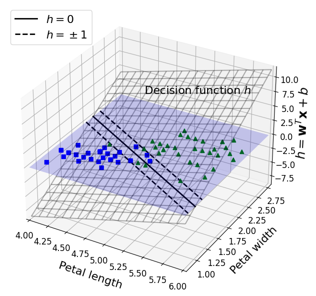
[그림 5-12]

[그림 5-12]: [그림 5-4] 오른쪽 모델의 결정 함수
- 특성이 두 개인 데이터셋으로 2차원 평면
- 결정 경계는 결정 함수의 값이 0인 점들로 이루어짐 => 두 평면의 교차점 (굵은 실선)
  - $n$ 개의 특성이 있을 때 결정함수는 $n$ 차원의 초평면, 결정 경계는 $(n-1)$ 차원의 초평면
점선은 결정 함수의 값이 1 또는 -1인 점들 => 결정 경계에 나란하고 일정한 거리만큼 떨어져서 마진을 형성
SVM 훈련: 마진 오류를 하나도 발생시키지 않거나 (하드 마진) 제한적인 마진 오류를 가지면서 (소프트 마진) 가능한 한 마진을 크게하는 $\mathbf{w}$ 와 $b$ 를 찾는 것

5.4.2 목적 함수

결정 함수의 기울기: 가중치 벡터의 노름 $\left \| \mathbf{w} \right \|$ 와 같음
- 기울기를 2로 나누면 결정 함수의 값이 $\pm 1$ 이 되는 점들이 결정 경계로부터 2배만큼 멀어짐 => 기울기의 1/2배는 마진에 2를 곱한것과 같다
- [그림 5-13] 에서 2차원 시각화 (가중치 벡터 $\mathbf{w}$ 가 작을수록 마진은 커짐)

<그림 5-13. 가중치 벡터가 작을수록 마진은 커집니다> 생성 코드

def plot_2D_decision_function(w, b, ylabel=True, x1_lim=[-3, 3]):
    x1 = np.linspace(x1_lim[0], x1_lim[1], 200)
    y = w * x1 + b
    m = 1 / w

    plt.plot(x1, y)
    plt.plot(x1_lim, [1, 1], "k:")
    plt.plot(x1_lim, [-1, -1], "k:")
    plt.axhline(y=0, color='k')
    plt.axvline(x=0, color='k')
    plt.plot([m, m], [0, 1], "k--")
    plt.plot([-m, -m], [0, -1], "k--")
    plt.plot([-m, m], [0, 0], "k-o", linewidth=3)
    plt.axis(x1_lim + [-2, 2])
    plt.xlabel(r"$x_1$", fontsize=16)
    if ylabel:
        plt.ylabel(r"$w_1 x_1$  ", rotation=0, fontsize=16)
    plt.title(r"$w_1 = {}$".format(w), fontsize=16)

fig, axes = plt.subplots(ncols=2, figsize=(9, 3.2), sharey=True)
plt.sca(axes[0])
plot_2D_decision_function(1, 0)
plt.sca(axes[1])
plot_2D_decision_function(0.5, 0, ylabel=False)
save_fig("small_w_large_margin_plot")
plt.show()

그림 저장: small_w_large_margin_plot

png

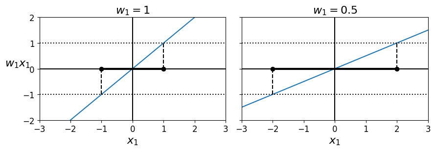
[그림 5-13]

마진을 크게 하기 위해 $\left \| \mathbf{w} \right \|$ 를 최소화
- 하드 마진: 모든 양성 훈련 샘플 1보다 커야하고, 음성 훈련 샘플은 -1보다 작아야 함
식 5-3: 하드 마진 선형 SVM 분류기 목적 함수 \[\begin{split} &\underset{\mathbf{w}, b}{\operatorname{minimize}}\quad{\frac{1}{2}\mathbf{w}^T \mathbf{w}} \\ &\text{subject to} \quad t^{(i)}(\mathbf{w}^T \mathbf{x}^{(i)} + b) \ge 1 \quad \text{for } i = 1, 2, \dots, m \end{split}\]

NOTE
$\left \| \mathbf{w} \right \|$ 를 최소화하는 대신 $\frac{1}{2}\left \| \mathbf{w} \right \|^{2}$ 인 $\frac{1}{2}\mathbf{w}^T \mathbf{w}$ 를 최소화
$\frac{1}{2}\left \| \mathbf{w} \right \|^{2}$ 는 미분 가능하지만 $\left \| \mathbf{w} \right \|$ 는 미분 불가능 ($\mathbf{w} = 0$ 에서)
최적화 알고리즘은 미분 가능한 함수에서 잘 작동

from sklearn.svm import SVC
from sklearn import datasets

iris = datasets.load_iris()
X = iris["data"][:, (2, 3)] # 꽃잎 길이, 꽃잎 너비
y = (iris["target"] == 2).astype(np.float64) # Iris virginica

svm_clf = SVC(kernel="linear", C=1)
svm_clf.fit(X, y)
svm_clf.predict([[5.3, 1.3]])

array([1.])

소프트 마진 분류기의 목적 함수 구성하려면 각 샘플에 개해 슬랙 변수 $\zeta^{(i)} \ge 0$ 을 도입해야 함
- $\zeta^{(i)}$ : $i$ 번째 샘플이 얼마나 마진을 위반할지 정함
마진 오류 최소화를 위한 슬랙 변수의 값을 작게 만드는 것과 마진을 크게하기 위해 $\frac{1}{2}\mathbf{w}^T \mathbf{w}$ 를 가능한 한 작게 만드는 목표 충돌
- 하이퍼파라미터 C: 두 목표 사이의 트레이드오프 정의
식 5-4: 소프트 마진 선형 SVM 분류기 목적 함수 \[\begin{split} &\underset{\mathbf{w}, b, \mathbf{\zeta}}{\operatorname{minimize}}\quad{\dfrac{1}{2}\mathbf{w}^T \mathbf{w} + C \sum\limits_{i=1}^m{\zeta^{(i)}}}\\ &\text{subject to} \quad t^{(i)}(\mathbf{w}^T \mathbf{x}^{(i)} + b) \ge 1 - \zeta^{(i)} \quad \text{and} \quad \zeta^{(i)} \ge 0 \quad \text{for } i = 1, 2, \dots, m \end{split}\]

5.4.3 콰드라틱 프로그래밍

하드 마진, 소프트 마진 문제 모두 선형적인 제약 조건이 있는 볼록 함수의 이차 최적화 문제 => 콰드라틱 프로그래밍(QP)
- 하드 마진 선형 SVM 분류기를 훈련시키는 한 가지 방법: 이미 준비되어 있는 QP 알고리즘에 관련 파라미터 전달
- 소프트 마진 문제에서도 QP 알고리즘 사용 가능 (연습 문제 참고)
- 커널 트릭을 사용하려면 제약이 있는 최적화 문제를 다른 형태로 변경해야함

5.4.4 쌍대 문제

원 문제 (primal problem) 라는 제약이 있는 최적화 문제가 주어지면 쌍대 문제 (dual problem) 라고 하는 깊게 관련된 다른 문제로 표현 가능
- 일반적으로 쌍대 문제 해는 원 문제 해의 하한값이지만, 어떤 조건하에서 원문제와 똑같은 해를 제공
- SVM 문제는 이 조건을 만족 (목적 함수 볼록, 부등식 제약 조건이 연속 미분 가능하면서 볼록 함수) => 원 문제 또는 쌍대 문제 중 하나 선택하여 풀 수 있음 (둘 다 같은 해 제공)
  - LinearSVC, LinearSVR 의 매개변수 dual 의 기본값 True를 False로 바꾸면 원 문제 선택 (SVC, SVR 은 쌍대 문제 만을 품)
훈련 샘플의 수 < 특성의 개수: 원 문제보다 쌍대 문제를 푸는 것이 더 빠름
- 원 문제에서는 적용이 안되는 커널 트릭 가능하게 함

5.4.5 커널 SVM

식 5-8: 2차 다항식 매핑 \[\phi\left(\mathbf{x}\right) = \phi\left( \begin{pmatrix} x_1 \\ x_2 \end{pmatrix} \right) = \begin{pmatrix} {x_1}^2 \\ \sqrt{2} \, x_1 x_2 \\ {x_2}^2 \end{pmatrix}\]

$\phi$ : 2차 다항식 매핑 함수
변환된 벡터는 2차원이 아닌 3차원이 됨

식 5-9: 2차 다항식 매핑을 위한 커널 트릭 \[\begin{split} \phi(\mathbf{a})^T \phi(\mathbf{b}) & \quad = \begin{pmatrix} {a_1}^2 \\ \sqrt{2} \, a_1 a_2 \\ {a_2}^2 \end{pmatrix}^T \begin{pmatrix} {b_1}^2 \\ \sqrt{2} \, b_1 b_2 \\ {b_2}^2 \end{pmatrix} = {a_1}^2 {b_1}^2 + 2 a_1 b_1 a_2 b_2 + {a_2}^2 {b_2}^2 \\ & \quad = \left( a_1 b_1 + a_2 b_2 \right)^2 = \left( \begin{pmatrix} a_1 \\ a_2 \end{pmatrix}^T \begin{pmatrix} b_1 \\ b_2 \end{pmatrix} \right)^2 = (\mathbf{a}^T \mathbf{b})^2 \end{split}\]

두 개의 2차원 벡터 $a$ 와 $b$ 에 2차 다항식 매칭을 적용한 다음 변환된 벡터로 점곱을 수행 => 원래 벡터의 점곱의 제곱과 같아짐
핵심: 모든 훈련 샘플에 변환 $\phi$ 를 적용 => [식 5-8] 의 2차 다항식 변환이면 간단하게 위와 같이 변경 가능 (그래서 실제로 훈련 샘플 변환 필요가 없음)
전체 과정에 필요한 계산량 측면에서 효율적 => 커널 트릭

2차 다항식 커널 : $K(\mathbf{a}, \mathbf{b}) = (\mathbf{a}^T \mathbf{b})^{2}$
머신러닝에서 커널: 변환 $\phi$ 를 계산하지 않고(또는 $\phi$ 를 모르더라도) 원래 벡터 $\mathbf{a}$ 와 $\mathbf{b}$ 에 기반하여 $\phi(\mathbf{a})^T \phi(\mathbf{b})$ 를 계산할 수 있는 함수

식 5-10: 일반적인 커널 \[\begin{split} \text{선형:} & \quad K(\mathbf{a}, \mathbf{b}) = \mathbf{a}^T \mathbf{b} \\ \text{다항식:} & \quad K(\mathbf{a}, \mathbf{b}) = \left(\gamma \mathbf{a}^T \mathbf{b} + r \right)^d \\ \text{가우시안 RBF:} & \quad K(\mathbf{a}, \mathbf{b}) = \exp({\displaystyle -\gamma \left\| \mathbf{a} - \mathbf{b} \right\|^2}) \\ \text{시그모이드:} & \quad K(\mathbf{a}, \mathbf{b}) = \tanh\left(\gamma \mathbf{a}^T \mathbf{b} + r\right) \end{split}\]

머서의 정리
머서의 조건: $K$ 가 매개변수에 대해 연속, 대칭
함수 $K(\mathbf{a}, \mathbf{b})$ 가 머서의 조건이라 불리는 몇개의 수학적 조건을 만족할 때, $a$ 와 $b$ 를 (더 높은 차원의) 다른 공간에 매핑하는 함수 $\phi$ 가 존재
가우시안 RBF 커널 => 각 훈련 샘플을 무한 차원의 공간에 매핑하는 것으로 볼 수 있음

커널 트릭을 사용한다면 $\phi\left(x^{(i)} \right)$ 를 포함 시켜야한다 => $\hat{\mathbf{w}}$ 의 차원이 매우 크거나 무한한 $\phi\left(x^{(i)} \right)$ 의 차원과 같아져야 하므로 계산 불가능
- [식 5-7] 의 $\hat{\mathbf{w}}$ 에 대한 식을 새로운 샘플 $\mathbf{x}^{(n)}$ 의 결정 함수에 적용하여 입력 벡터 간의 점곱으로만된 식을 얻을 수 있음 ($\hat{\mathbf{w}}$ 모른채 예측 가능)
- 서포트 벡터만 $\alpha^{(i)} \neq 0$ 이기 때문에 예측을 만드는 데는 서포트 벡터와 새로운 입력 벡터 $\mathbf{x}^{(n)}$ 간의 점곱만 계산하면 됨 (물론 편향 $\hat{b}$ 도 커널 트릭으로 계산해야 함)
- [식 5-7]: 쌍대 문제에서 구한 해로 원 문제의 해 계산하는 식

5.4.6 온라인 SVM

식 5-13: 선형 SVM 분류기의 비용 함수 \[J(\mathbf{w}, b) = \dfrac{1}{2} \mathbf{w}^T \mathbf{w} \,+\, C {\displaystyle \sum\limits_{i=1}^{m}max\left(0, t^{(i)} - (\mathbf{w}^T \mathbf{x}^{(i)} + b) \right)}\]

온라인 SVM 분류기를 구현하는 한가지 방법: 원 문제로부터 유도된 [식 5-13] 의 비용함수를 최소화하기 위한 경사 하강법을 사용하는 것 (ex: SGDClassifier에서 loss 매개변수를 기본값인 hinge로 지정하면 선형 SVM 문제가 됨)
첫 번째 항: 모델이 작은 가중치 벡터 $\mathbf{w}$ 를 가지도록 제약을 가해 마진을 크게 만듦
두 번째 항: 모든 마진 오류 계산
- 이 항을 최소화하면 마진 오류를 가능한 줄이고 크기도 작게 만듦

힌지 손실
힌지 손실 함수: $\max(0, 1-t)$
이 함수는 $t=1$ 에서 미분 불가능이지만, 라쏘 회귀처럼 $t=1$ 에서 서브그레이디언트 를 사용해 경사 하강법 사용 가능 (즉, -1과 0사이의 값을 사용) => SGDClassifier 의 힌지 손실 함수는 $t=1$ 일 때 -1 사용

힌지 손실 그림 생성 코드

t = np.linspace(-2, 4, 200)
h = np.where(1 - t < 0, 0, 1 - t)  # max(0, 1-t)

plt.figure(figsize=(5,2.8))
plt.plot(t, h, "b-", linewidth=2, label="$max(0, 1 - t)$")
plt.grid(True, which='both')
plt.axhline(y=0, color='k')
plt.axvline(x=0, color='k')
plt.yticks(np.arange(-1, 2.5, 1))
plt.xlabel("$t$", fontsize=16)
plt.axis([-2, 4, -1, 2.5])
plt.legend(loc="upper right", fontsize=16)
save_fig("hinge_plot")
plt.show()

그림 저장: hinge_plot

png

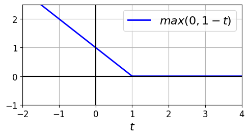
힌지 손실 함수

온라인 커널 SVM을 구현하는 것도 가능
- 「Incremental and Decremental Support Vector Machine Learning」이나 「Fast Kernel Classifiers With Online and Active Learning」과 같은 논문에 기술된 온라인 커널 SVM을 구현할 수도 있음
  - 하지만, 이 커널 SVM들은 Matlab이나 C++로 구현됨
대규모의 비선형 문제라면 신경망 알고리즘 고려하는 것이 좋음 (2부 참조)

추가 내용

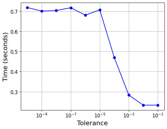
훈련 시간

X, y = make_moons(n_samples=1000, noise=0.4, random_state=42)
plt.plot(X[:, 0][y==0], X[:, 1][y==0], 'bs')
plt.plot(X[:, 0][y==1], X[:, 1][y==1], 'g^')

[<matplotlib.lines.Line2D at 0x233598e6148>]

png

import time

tol = 0.1
tols = []
times = []
for i in range(10):
    svm_clf = SVC(kernel="poly", gamma=3, C=10, tol=tol, verbose=1)
    t1 = time.time()
    svm_clf.fit(X, y)
    t2 = time.time()
    times.append(t2-t1)
    tols.append(tol)
    print(i, tol, t2-t1)
    tol /= 10
plt.semilogx(tols, times, "bo-")
plt.xlabel("Tolerance", fontsize=16)
plt.ylabel("Time (seconds)", fontsize=16)
plt.grid(True)
plt.show()

[LibSVM]0 0.1 0.23304295539855957
[LibSVM]1 0.01 0.23305225372314453
[LibSVM]2 0.001 0.2830631732940674
[LibSVM]3 0.0001 0.4701056480407715
[LibSVM]4 1e-05 0.7071585655212402
[LibSVM]5 1.0000000000000002e-06 0.6811525821685791
[LibSVM]6 1.0000000000000002e-07 0.7181613445281982
[LibSVM]7 1.0000000000000002e-08 0.7041678428649902
[LibSVM]8 1.0000000000000003e-09 0.7011570930480957
[LibSVM]9 1.0000000000000003e-10 0.7191519737243652

png

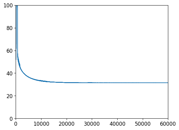
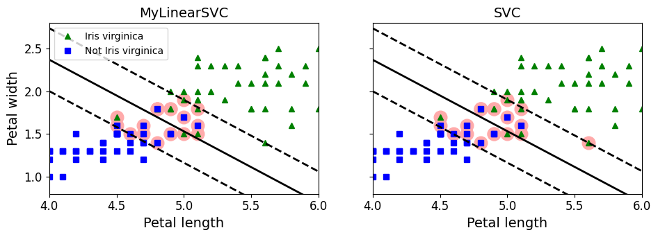
배치 경사 하강법을 사용한 선형 SVM 분류기 구현

# 훈련 세트
X = iris["data"][:, (2, 3)] # # 꽃잎 길이, 꽃잎 너비
y = (iris["target"] == 2).astype(np.float64).reshape(-1, 1) # Iris virginica

from sklearn.base import BaseEstimator

class MyLinearSVC(BaseEstimator):
    def __init__(self, C=1, eta0=1, eta_d=10000, n_epochs=1000, random_state=None):
        self.C = C
        self.eta0 = eta0
        self.n_epochs = n_epochs
        self.random_state = random_state
        self.eta_d = eta_d

    def eta(self, epoch):
        return self.eta0 / (epoch + self.eta_d)
        
    def fit(self, X, y):
        # Random initialization
        if self.random_state:
            np.random.seed(self.random_state)
        w = np.random.randn(X.shape[1], 1) # n feature weights
        b = 0

        m = len(X)
        t = y * 2 - 1  # -1 if y==0, +1 if y==1
        X_t = X * t
        self.Js=[]

        # Training
        for epoch in range(self.n_epochs):
            support_vectors_idx = (X_t.dot(w) + t * b < 1).ravel()
            X_t_sv = X_t[support_vectors_idx]
            t_sv = t[support_vectors_idx]

            J = 1/2 * np.sum(w * w) + self.C * (np.sum(1 - X_t_sv.dot(w)) - b * np.sum(t_sv))
            self.Js.append(J)

            w_gradient_vector = w - self.C * np.sum(X_t_sv, axis=0).reshape(-1, 1)
            b_derivative = -self.C * np.sum(t_sv)
                
            w = w - self.eta(epoch) * w_gradient_vector
            b = b - self.eta(epoch) * b_derivative
            

        self.intercept_ = np.array([b])
        self.coef_ = np.array([w])
        support_vectors_idx = (X_t.dot(w) + t * b < 1).ravel()
        self.support_vectors_ = X[support_vectors_idx]
        return self

    def decision_function(self, X):
        return X.dot(self.coef_[0]) + self.intercept_[0]

    def predict(self, X):
        return (self.decision_function(X) >= 0).astype(np.float64)

C=2
svm_clf = MyLinearSVC(C=C, eta0 = 10, eta_d = 1000, n_epochs=60000, random_state=2)
svm_clf.fit(X, y)
svm_clf.predict(np.array([[5, 2], [4, 1]]))

array([[1.],
       [0.]])

plt.plot(range(svm_clf.n_epochs), svm_clf.Js)
plt.axis([0, svm_clf.n_epochs, 0, 100])

(0.0, 60000.0, 0.0, 100.0)

png

print(svm_clf.intercept_, svm_clf.coef_)

[-15.56761653] [[[2.28120287]
  [2.71621742]]]

svm_clf2=SVC(kernel='linear', C=C)
svm_clf2.fit(X, y.ravel())
print(svm_clf2.intercept_, svm_clf2.coef_)

[-15.51721253] [[2.27128546 2.71287145]]

yr = y.ravel()
fig, axes = plt.subplots(ncols=2, figsize=(11, 3.2), sharey=True)
plt.sca(axes[0])
plt.plot(X[:, 0][yr==1], X[:, 1][yr==1], "g^", label="Iris virginica")
plt.plot(X[:, 0][yr==0], X[:, 1][yr==0], "bs", label="Not Iris virginica")
plot_svc_decision_boundary(svm_clf, 4, 6)
plt.xlabel("Petal length", fontsize=14)
plt.ylabel("Petal width", fontsize=14)
plt.title("MyLinearSVC", fontsize=14)
plt.axis([4, 6, 0.8, 2.8])
plt.legend(loc="upper left")

plt.sca(axes[1])
plt.plot(X[:, 0][yr==1], X[:, 1][yr==1], "g^")
plt.plot(X[:, 0][yr==0], X[:, 1][yr==0], "bs")
plot_svc_decision_boundary(svm_clf2, 4, 6)
plt.xlabel("Petal length", fontsize=14)
plt.title("SVC", fontsize=14)
plt.axis([4, 6, 0.8, 2.8])

(4.0, 6.0, 0.8, 2.8)

png

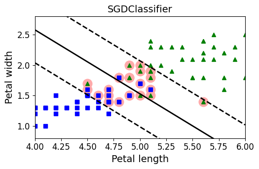
from sklearn.linear_model import SGDClassifier

sgd_clf = SGDClassifier(loss="hinge", alpha=0.017, max_iter=1000, tol=1e-3, random_state=42)
sgd_clf.fit(X, y.ravel())

m = len(X)
t = y * 2 - 1  # y==0이면 -1, y==1이면 +1
X_b = np.c_[np.ones((m, 1)), X]  # 편향 x0=1을 추가합니다
X_b_t = X_b * t
sgd_theta = np.r_[sgd_clf.intercept_[0], sgd_clf.coef_[0]]
print(sgd_theta)
support_vectors_idx = (X_b_t.dot(sgd_theta) < 1).ravel()
sgd_clf.support_vectors_ = X[support_vectors_idx]
sgd_clf.C = C

plt.figure(figsize=(5.5,3.2))
plt.plot(X[:, 0][yr==1], X[:, 1][yr==1], "g^")
plt.plot(X[:, 0][yr==0], X[:, 1][yr==0], "bs")
plot_svc_decision_boundary(sgd_clf, 4, 6)
plt.xlabel("Petal length", fontsize=14)
plt.ylabel("Petal width", fontsize=14)
plt.title("SGDClassifier", fontsize=14)
plt.axis([4, 6, 0.8, 2.8])

[-12.52988101   1.94162342   1.84544824]

(4.0, 6.0, 0.8, 2.8)

png

연습문제 풀이

서포트 벡터 머신의 근본 아이디어는 무엇인가요?
- 클래스 사이에 가능한 한 가장 넓은 ‘도로’를 내는 것 => 두 클래스를 구분하는 결정 경계와 샘플 사이의 마진을 가능한 가장 크게 하는 것
- 소프트 마진 분류: SVM이 두 클래스를 완벽하게 나누는 것과 가장 넓은 도로를 만드는 것 사이의 절충안 찾음 (몇 개의 샘플은 도로안에 있을 수 있음)
- 비선형 데이터셋에서 훈련할 때 커널 함수 사용하는 것
서포트 벡터가 무엇인가요?
- SVM이 훈련된 후에 경계를 포함해 도로에 놓인 어떤 샘플
- 결정 경계는 전적으로 서포트 벡터에 의해 결정
  - 서포트 벡터가 아닌 다른 샘플은 영향 주지 못함 => 이런 샘플은 다른 곳으로 이동시키거나 삭제하고 다른 샘플 더 추가할 수 있음
- 예측 계산에는 전체 훈련 세트가 아니라 서포트 벡터만 관여
SVM을 사용할 때 입력값의 스케일이 왜 중요한가요?
- 클래스 사이에 가능한 한 큰 도로를 내는 것이므로 훈련 스케일이 맞지않으면 크기가 작은 특성을 무시하는 경향이 있다
SVM 분류기가 샘플을 분류할 때 신뢰도 점수와 확률을 출력할 수 있나요?
- 테스트 샘플과 결정 경계사이의 거리를 출력할 수 있으므로 이를 신뢰도 점수로 활용 가능
- 이를 추정값으로 변환하기 위해 probability=True 로 설정하면 훈련이 끝난 후 (5-겹 교차검증을 추가로 훈련한) SVM의 점수에 로지스틱 회귀를 훈련시켜 확률 계산
  - 이 설정은 SVM 모델에 predict_proba() 와 predict_log_proba() 메서드 추가
  - 대신 훈련 속도가 느려지고, predict() 와 predict_proba()의 결과가 달라질 수 있음
수백만 개의 샘플과 수백 개의 특성을 가진 훈련 세트에 SVM 모델을 훈련시키려면 원 문제와 쌍대 문제 중 어떤 것을 사용해야 하나요?
- 쌍대 형식이 너무 느려지기 때문에 원 문제를 사용해야함
- 커널 SVM은 쌍대 형식만 사용 가능하므로 이 질문은 선형 SVM에만 해당
RBF 커널을 사용해 SVM 분류기를 훈련 시켰더니 훈련 세트에 과소적합된 것 같습니다. $\gamma$ (gamma)를 증가시켜야 할까요, 감소시켜야 할까요? ($C$ 의 경우는 어떤가요)
- 규제를 줄이기 위해 둘 중 하나를 증가 혹은 둘다 증가시켜야 함
이미 만들어진 QP 알고리즘 라이브러리를 사용해 소프트 마진 선형 SVM 분류기를 학습시키려면 QP 매개변수 ($\mathbf{H}, \mathbf{f}, \mathbf{A}, \mathbf{b}$) 를 어떻게 지정해야 하나요?
하드 마진에 대한 QP 파라미터 $\mathbf{H}', \mathbf{f}', \mathbf{A}', \mathbf{b}'$ 라고 설정, 소프트 마진 문제의 QP 파라미터는 $m$ 개의 추가적인 파라미터 ($n_p=n+1+m$) 와 $m$ 개의 추가적인 제약 ($n_c=2m$) 을 가짐
- $\mathbf{H}$: $\mathbf{H}'$ 의 오른쪽에 0으로 채워진 $m$개의 열이 있고 아래에 0으로 채워진 $m$개의 열이 있는 행렬
- $\mathbf{f}$: $\mathbf{f}'$ 에 하이퍼퍼라미터 $C$와 동일한 값의 원소 $m$ 개가 추가된 벡터
- $\mathbf{b}$: $\mathbf{b}'$ 에 값이 0인 원소 $m$ 개가 추가된 벡터
- $\mathbf{A}$: $\mathbf{A}'$ 의 오른쪽에서 $-\mathbf{I}_m$ 이 추가되고 바로 그 아래에 $-\mathbf{I}_m$ 이 추가되며 나머지는 0으로 채워진 행렬 ($\mathbf{I}_m$ 은 $m \times n$ 단위 행렬)
선형적으로 분리되는 데이터셋에 LinearSVC를 훈련시켜보세요. 그런 다음 같은 데이터셋에 SVC와 SGDClassifier를 적용해보세요. 거의 비슷한 모델이 만들어지는지 확인해보세요.

Iris 데이터셋을 사용( Iris Setosa와 Iris Versicolor 클래스는 선형적으로 구분이 가능)

from sklearn import datasets

iris=datasets.load_iris()
X=iris['data'][:,(2,3)] # 꽃잎 길이, 꽃잎 너비
y=iris['target']

setosa_or_versicolor = (y == 0) | (y == 1)
X = X[setosa_or_versicolor]
y = y[setosa_or_versicolor]

from sklearn.svm import SVC, LinearSVC
from sklearn.linear_model import SGDClassifier
from sklearn.preprocessing import StandardScaler

C=5
alpha=1/(C*len(X))

lin_clf=LinearSVC(loss='hinge', C=C, random_state=42)
svm_clf=SVC(kernel='linear', C=C)
sgd_clf=SGDClassifier(loss='hinge', learning_rate='constant', eta0=0.001, alpha=alpha,
                     max_iter=1000, tol=1e-3, random_state=42)

scaler=StandardScaler()
X_scaled=scaler.fit_transform(X)

lin_clf.fit(X_scaled, y)
svm_clf.fit(X_scaled, y)
sgd_clf.fit(X_scaled, y)

print("LinearSVC:                   ", lin_clf.intercept_, lin_clf.coef_)
print("SVC:                         ", svm_clf.intercept_, svm_clf.coef_)
print("SGDClassifier(alpha={:.5f}):".format(sgd_clf.alpha), sgd_clf.intercept_, sgd_clf.coef_)

LinearSVC:                    [0.28475098] [[1.05364854 1.09903804]]
SVC:                          [0.31896852] [[1.1203284  1.02625193]]
SGDClassifier(alpha=0.00200): [0.117] [[0.77714169 0.72981762]]

이 3개 모델의 결정 경계:

# 각 결정 경계의 기울기와 편향을 계산
w1 = -lin_clf.coef_[0, 0]/lin_clf.coef_[0, 1]
b1 = -lin_clf.intercept_[0]/lin_clf.coef_[0, 1]
w2 = -svm_clf.coef_[0, 0]/svm_clf.coef_[0, 1]
b2 = -svm_clf.intercept_[0]/svm_clf.coef_[0, 1]
w3 = -sgd_clf.coef_[0, 0]/sgd_clf.coef_[0, 1]
b3 = -sgd_clf.intercept_[0]/sgd_clf.coef_[0, 1]

# 결정 경계를 원본 스케일로 변환
line1 = scaler.inverse_transform([[-10, -10 * w1 + b1], [10, 10 * w1 + b1]])
line2 = scaler.inverse_transform([[-10, -10 * w2 + b2], [10, 10 * w2 + b2]])
line3 = scaler.inverse_transform([[-10, -10 * w3 + b3], [10, 10 * w3 + b3]])

# 세 개의 결정 경계
plt.figure(figsize=(11, 4))
plt.plot(line1[:, 0], line1[:, 1], "k:", label="LinearSVC")
plt.plot(line2[:, 0], line2[:, 1], "b--", linewidth=2, label="SVC")
plt.plot(line3[:, 0], line3[:, 1], "r-", label="SGDClassifier")
plt.plot(X[:, 0][y==1], X[:, 1][y==1], "bs") # label="Iris versicolor"
plt.plot(X[:, 0][y==0], X[:, 1][y==0], "yo") # label="Iris setosa"
plt.xlabel("Petal length", fontsize=14)
plt.ylabel("Petal width", fontsize=14)
plt.legend(loc="upper center", fontsize=14)
plt.axis([0, 5.5, 0, 2])

plt.show()

png

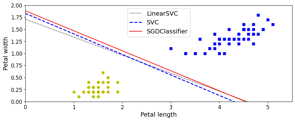
아주 비슷하다

9. MNIST 데이터셋에 SVM 분류기를 훈련시켜보세요. SVM 분류기는 이진 분류기라서 OvA (OvR)전략을 사용해 10개의 숫자를 분류해야 합니다. 처리 속도를 높이기 위해 작은 검증 세트로 하이퍼파라미터를 조정하는 것이 좋습니다. 어느 정도까지 정확도를 높일 수 있나요?

먼저 데이터셋을 로드하고 훈련 세트와 테스트 세트로 나눕니다. train_test_split() 함수를 사용할 수 있지만 보통 처음 60,000개의 샘플을 훈련 세트로 사용하고 나머지는 10,000개를 테스트 세트로 사용합니다(이렇게 하면 다른 사람들의 모델과 성능을 비교하기 좋습니다):

from sklearn.datasets import fetch_openml
mnist=fetch_openml('mnist_784', version=1, cache=True)

X=mnist['data']
y=mnist['target'].astype(np.uint8)

X_train = X[:60000]
y_train = y[:60000]
X_test = X[60000:]
y_test = y[60000:]

많은 훈련 알고리즘은 훈련 샘플의 순서에 민감하므로 먼저 이를 섞는 것이 좋은 습관이지만 이 데이터셋은 이미 섞여있으므로 이렇게 할 필요가 없다

선형 SVM 분류기: 자동으로 OvA(또는 OvR) 전략을 사용하므로 특별히 처리해 줄 것이 없다

lin_clf=LinearSVC(random_state=42)
lin_clf.fit(X_train, y_train)

C:\Users\pjj11\anaconda3\envs\test3.7\lib\site-packages\sklearn\svm\_base.py:1208: ConvergenceWarning: Liblinear failed to converge, increase the number of iterations.
  ConvergenceWarning,

LinearSVC(random_state=42)

훈련 세트에 대한 예측을 만들어 정확도를 측정(최종 모델을 선택해 훈련시킨 것이 아니기 때문에 아직 테스트 세트를 사용해서는 안됨):

from sklearnlearn.metrics import accuracy_score

y_pred = lin_clf.predict(X_train)
accuracy_score(y_train, y_pred)

0.8348666666666666

MNIST에서 83.5% 정확도면 나쁜 성능 => 선형 모델이 MNIST 문제에 너무 단순하기 때문이지만 먼저 데이터의 스케일을 조정할 필요가 있다:

scaler = StandardScaler()
X_train_scaled = scaler.fit_transform(X_train.astype(np.float32))
X_test_scaled = scaler.transform(X_test.astype(np.float32))

lin_clf = LinearSVC(random_state=42)
lin_clf.fit(X_train_scaled, y_train)

C:\Users\pjj11\anaconda3\envs\test3.7\lib\site-packages\sklearn\svm\_base.py:1208: ConvergenceWarning: Liblinear failed to converge, increase the number of iterations.
  ConvergenceWarning,

LinearSVC(random_state=42)

y_pred = lin_clf.predict(X_train_scaled)
accuracy_score(y_train, y_pred)

0.9214

훨씬 나아졌지만(에러율을 절반으로 줄임) 여전히 MNIST에서 좋은 성능은 아니다. SVM을 사용한다면 커널 함수를 사용해야 합니다. RBF 커널(기본값)로 SVC를 적용:

노트: 향후 버전을 위해 사이킷런 0.22에서 기본값인 gamma="scale"을 지정

svm_clf = SVC(gamma="scale")
svm_clf.fit(X_train_scaled[:10000], y_train[:10000])

SVC()

y_pred = svm_clf.predict(X_train_scaled)
accuracy_score(y_train, y_pred)

0.9455333333333333

6배나 적은 데이터에서 모델을 훈련시켰지만 더 좋은 성능을 얻었다. 교차 검증을 사용한 랜덤 서치로 하이퍼파라미터 튜닝(진행을 빠르게 하기 위해 작은 데이터셋으로 작업):

from sklearn.model_selection import RandomizedSearchCV
from scipy.stats import reciprocal, uniform

param_distributions = {"gamma": reciprocal(0.001, 0.1), "C": uniform(1, 10)}
rnd_search_cv = RandomizedSearchCV(svm_clf, param_distributions, n_iter=10, verbose=2, cv=3)
rnd_search_cv.fit(X_train_scaled[:1000], y_train[:1000])

Fitting 3 folds for each of 10 candidates, totalling 30 fits
[CV] END ....C=5.847490967837556, gamma=0.004375955271336425; total time=   0.1s
[CV] END ....C=5.847490967837556, gamma=0.004375955271336425; total time=   0.1s
[CV] END ....C=5.847490967837556, gamma=0.004375955271336425; total time=   0.1s
[CV] END ....C=2.544266730893301, gamma=0.024987648190235304; total time=   0.1s
[CV] END ....C=2.544266730893301, gamma=0.024987648190235304; total time=   0.1s
[CV] END ....C=2.544266730893301, gamma=0.024987648190235304; total time=   0.1s
[CV] END ....C=2.199505425963898, gamma=0.009340106304825553; total time=   0.1s
[CV] END ....C=2.199505425963898, gamma=0.009340106304825553; total time=   0.1s
[CV] END ....C=2.199505425963898, gamma=0.009340106304825553; total time=   0.1s
[CV] END .....C=7.327377306009368, gamma=0.04329656504133618; total time=   0.1s
[CV] END .....C=7.327377306009368, gamma=0.04329656504133618; total time=   0.1s
[CV] END .....C=7.327377306009368, gamma=0.04329656504133618; total time=   0.1s
[CV] END ....C=7.830259944094713, gamma=0.009933958471354695; total time=   0.1s
[CV] END ....C=7.830259944094713, gamma=0.009933958471354695; total time=   0.1s
[CV] END ....C=7.830259944094713, gamma=0.009933958471354695; total time=   0.1s
[CV] END ....C=6.867969780001033, gamma=0.027511132256566175; total time=   0.1s
[CV] END ....C=6.867969780001033, gamma=0.027511132256566175; total time=   0.1s
[CV] END ....C=6.867969780001033, gamma=0.027511132256566175; total time=   0.1s
[CV] END .....C=3.584980864373988, gamma=0.01237128009623357; total time=   0.1s
[CV] END .....C=3.584980864373988, gamma=0.01237128009623357; total time=   0.1s
[CV] END .....C=3.584980864373988, gamma=0.01237128009623357; total time=   0.1s
[CV] END ....C=5.073078322899452, gamma=0.002259275783824143; total time=   0.1s
[CV] END ....C=5.073078322899452, gamma=0.002259275783824143; total time=   0.1s
[CV] END ....C=5.073078322899452, gamma=0.002259275783824143; total time=   0.1s
[CV] END ..C=10.696324058267928, gamma=0.0039267813006514255; total time=   0.1s
[CV] END ..C=10.696324058267928, gamma=0.0039267813006514255; total time=   0.1s
[CV] END ..C=10.696324058267928, gamma=0.0039267813006514255; total time=   0.1s
[CV] END ..C=3.8786881587000437, gamma=0.0017076019229344522; total time=   0.1s
[CV] END ..C=3.8786881587000437, gamma=0.0017076019229344522; total time=   0.1s
[CV] END ..C=3.8786881587000437, gamma=0.0017076019229344522; total time=   0.1s





RandomizedSearchCV(cv=3, estimator=SVC(),
                   param_distributions={'C': <scipy.stats._distn_infrastructure.rv_frozen object at 0x0000019499A59A48>,
                                        'gamma': <scipy.stats._distn_infrastructure.rv_frozen object at 0x0000019499A59DC8>},
                   verbose=2)

rnd_search_cv.best_estimator_

SVC(C=3.8786881587000437, gamma=0.0017076019229344522)

rnd_search_cv.best_score_

0.8599947252641863

이 점수는 낮지만 1,000개의 샘플만 사용한 것을 기억해야 함 => 전체 데이터셋으로 최선의 모델을 재훈련:

rnd_search_cv.best_estimator_.fit(X_train_scaled, y_train)

SVC(C=3.8786881587000437, gamma=0.0017076019229344522)

y_pred = rnd_search_cv.best_estimator_.predict(X_train_scaled)
accuracy_score(y_train, y_pred)

0.9978166666666667

이제 이 모델을 선택하여 테스트 세트로 모델을 테스트:

y_pred = rnd_search_cv.best_estimator_.predict(X_test_scaled)
accuracy_score(y_test, y_pred)

0.9717

아주 나쁘지 않지만 확실히 모델이 다소 과대적합되었다. 하이퍼파라미터를 조금 더 수정할 수 있지만(가령, C와/나 gamma를 감소시킵니다) 그렇게 하면 테스트 세트에 과대적합될 위험이 있다.
다른 사람들은 하이퍼파라미터 C=5와 gamma=0.005에서 더 나은 성능(98% 이상의 정확도)을 얻었다. 훈련 세트를 더 많이 사용해서 더 오래 랜덤 서치를 수행하면 이런 값을 얻을 수 있을지 모른다.

10. 문제: 캘리포니아 주택 가격 데이터셋에 SVM 회귀를 훈련시켜보세요.

사이킷런의 fetch_california_housing() 함수를 사용해 데이터셋을 로드:

from sklearn.datasets import fetch_california_housing

housing=fetch_california_housing()
X=housing['data']
y=housing['target']

훈련 세트와 테스트 세트로 나눔:

from sklearn.model_selection import train_test_split

X_train, X_test, y_train, y_test=train_test_split(X, y, test_size=0.2, random_state=42)

데이터의 스케일을 조정:

from sklearn.preprocessing import StandardScaler

scaler=StandardScaler()
X_train_scaled=scaler.fit_transform(X_train)
X_test_scaled=scaler.transform(X_test)

먼저 간단한 LinearSVR을 훈련:

from sklearn.svm import LinearSVR

lin_reg=LinearSVR(random_state=42)
lin_reg.fit(X_train_scaled, y_train)

C:\Users\pjj11\anaconda3\envs\test3.7\lib\site-packages\sklearn\svm\_base.py:1208: ConvergenceWarning: Liblinear failed to converge, increase the number of iterations.
  ConvergenceWarning,

LinearSVR(random_state=42)

훈련 세트에 대한 성능을 확인(RMSE):

from sklearn.metrics import mean_squared_error

y_pred=lin_reg.predict(X_train_scaled)
mse=mean_squared_error(y_train, y_pred)
rmse=np.sqrt(mse)
rmse

0.9819256687727764

훈련 세트에서 타깃은 만달러 단위이다.
RMSE는 기대할 수 있는 에러의 정도를 대략 가늠하게 도와준다(에러가 클수록 큰 폭으로 증가).
이 모델의 에러가 대략 $10,000 정도로 예상할 수 있다.

RBF 커널이 더 나을지 확인 => 하이퍼파라미터 C와 gamma의 적절한 값을 찾기 위해 교차 검증을 사용한 랜덤 서치를 적용:

from sklearn.svm import SVR
from sklearn.model_selection import RandomizedSearchCV
from scipy.stats import reciprocal, uniform

param_distributions={'gamma':reciprocal(0.001, 0.1), 'C':uniform(1,10)}
rnd_search_cv=RandomizedSearchCV(SVR(), param_distributions, n_iter=10, verbose=2, cv=3, random_state=42)
rnd_search_cv.fit(X_train_scaled, y_train)

Fitting 3 folds for each of 10 candidates, totalling 30 fits
[CV] END .....C=4.745401188473625, gamma=0.07969454818643928; total time=   9.1s
[CV] END .....C=4.745401188473625, gamma=0.07969454818643928; total time=   9.1s
[CV] END .....C=4.745401188473625, gamma=0.07969454818643928; total time=   9.1s
[CV] END .....C=8.31993941811405, gamma=0.015751320499779724; total time=   9.1s
[CV] END .....C=8.31993941811405, gamma=0.015751320499779724; total time=   8.9s
[CV] END .....C=8.31993941811405, gamma=0.015751320499779724; total time=   9.0s
[CV] END ....C=2.560186404424365, gamma=0.002051110418843397; total time=   8.8s
[CV] END ....C=2.560186404424365, gamma=0.002051110418843397; total time=   8.9s
[CV] END ....C=2.560186404424365, gamma=0.002051110418843397; total time=   9.0s
[CV] END ....C=1.5808361216819946, gamma=0.05399484409787431; total time=   8.6s
[CV] END ....C=1.5808361216819946, gamma=0.05399484409787431; total time=   8.6s
[CV] END ....C=1.5808361216819946, gamma=0.05399484409787431; total time=   8.6s
[CV] END ....C=7.011150117432088, gamma=0.026070247583707663; total time=   8.9s
[CV] END ....C=7.011150117432088, gamma=0.026070247583707663; total time=   9.0s
[CV] END ....C=7.011150117432088, gamma=0.026070247583707663; total time=   9.1s
[CV] END .....C=1.2058449429580245, gamma=0.0870602087830485; total time=   8.5s
[CV] END .....C=1.2058449429580245, gamma=0.0870602087830485; total time=   8.5s
[CV] END .....C=1.2058449429580245, gamma=0.0870602087830485; total time=   8.5s
[CV] END ...C=9.324426408004218, gamma=0.0026587543983272693; total time=   9.0s
[CV] END ...C=9.324426408004218, gamma=0.0026587543983272693; total time=   8.9s
[CV] END ...C=9.324426408004218, gamma=0.0026587543983272693; total time=   8.9s
[CV] END ...C=2.818249672071006, gamma=0.0023270677083837795; total time=   8.9s
[CV] END ...C=2.818249672071006, gamma=0.0023270677083837795; total time=   8.9s
[CV] END ...C=2.818249672071006, gamma=0.0023270677083837795; total time=   8.9s
[CV] END ....C=4.042422429595377, gamma=0.011207606211860567; total time=   8.8s
[CV] END ....C=4.042422429595377, gamma=0.011207606211860567; total time=   8.8s
[CV] END ....C=4.042422429595377, gamma=0.011207606211860567; total time=   8.8s
[CV] END ....C=5.319450186421157, gamma=0.003823475224675185; total time=   8.8s
[CV] END ....C=5.319450186421157, gamma=0.003823475224675185; total time=   8.9s
[CV] END ....C=5.319450186421157, gamma=0.003823475224675185; total time=   8.9s





RandomizedSearchCV(cv=3, estimator=SVR(),
                   param_distributions={'C': <scipy.stats._distn_infrastructure.rv_frozen object at 0x00000194128C3DC8>,
                                        'gamma': <scipy.stats._distn_infrastructure.rv_frozen object at 0x00000194126FEFC8>},
                   random_state=42, verbose=2)

rnd_search_cv.best_estimator_

SVR(C=4.745401188473625, gamma=0.07969454818643928)

이제 훈련 세트에서 RMSE를 측정:

y_pred=rnd_search_cv.best_estimator_.predict(X_train_scaled)
mse=mean_squared_error(y_train, y_pred)
np.sqrt(mse)

0.5727524770785372

선형 모델보다 훨씬 나아졌다 => 이 모델을 선택하고 테스트 세트에서 평가:

y_pred=rnd_search_cv.best_estimator_.predict(X_test_scaled)
mse=mean_squared_error(y_test, y_pred)
np.sqrt(mse)

0.5929168385528758

출처

핸즈온 머신러닝 2판

5. 서포트 벡터 머신

설정

5.1 선형 SVM 분류

5.1.1 소프트 마진 분류

5.2 비선형 SVM 분류

5.2.1 다항식 커널

5.2.2 유사도 측정

5.2.3 가우시안 RBF 커널

5.2.4 계산 복잡도

5.3 SVM 회귀

5.4 SVM 이론

5.4.1 결정 함수와 예측

5.4.2 목적 함수

5.4.3 콰드라틱 프로그래밍

5.4.4 쌍대 문제

5.4.5 커널 SVM

5.4.6 온라인 SVM

추가 내용

훈련 시간

배치 경사 하강법을 사용한 선형 SVM 분류기 구현

연습문제 풀이

출처

pjj11005

Error

파이썬 클래스	시간 복잡도	외부 메모리 학습 지원	스케일 조정 필요성	커널 트릭
`LinearSVC`	\(O(m \times n)\)	아니오	예	아니오
`SGDClassifier`	\(O(m \times n)\)	예	예	아니오
`SVC`	\(O(m^{2} \times n)\) ~ \(O(m^{3} \times n)\)	아니오	예	예

설정

5.1 선형 SVM 분류

5.1.1 소프트 마진 분류

5.2 비선형 SVM 분류

5.2.1 다항식 커널

5.2.2 유사도 측정

5.2.3 가우시안 RBF 커널

5.2.4 계산 복잡도

5.3 SVM 회귀

5.4 SVM 이론

5.4.1 결정 함수와 예측

5.4.2 목적 함수

5.4.3 콰드라틱 프로그래밍

5.4.4 쌍대 문제

5.4.5 커널 SVM

5.4.6 온라인 SVM

추가 내용

훈련 시간

배치 경사 하강법을 사용한 선형 SVM 분류기 구현

연습문제 풀이

출처

Templates (for web app):

Error